Tags & Description
Explain the definitions for each
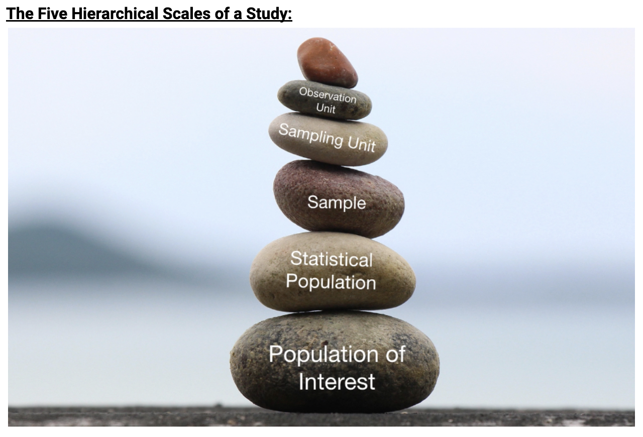
Definitions
Sampling unit: The unit that is selected at random. Ie if you randomly selecting 100 email adresses to find favouite grocery store; the sampling unit would be the email address of a person. Note sample unit could be the same as the observation unit
Sample: The collection of all sampling units that were randomly selected. ie if only 50 people replied to your email with an answer, then your sample is 50 email responses.
Statistical population: The collection of all sampling units that could have been selected to be in your sample. The statistical problem is defined by your study design. It represents the true scale in which your statistical conclusions are valid. Ie you collected data by sending emails to 100 random people from a list of email addresses residing in Toronto. The statistical population would be all people in Toronto with and active email account.
Population of interest: The population(the collection of sampling units) that you hope to draw a conclusion about. Ideally, the population of interest is the same as your statistical population. The population of interest is defined by the question being answered by your study. Ie if the question being answered was; ‘do more people shop at large grocery stores as appose to local grocery/convience stores?’: then the population of interest would be all people living in Toronto.
Observation unit: The unit you (directly) collect data from. This can sometimes be the same as the sampling unit. But most often they are not the same. The observation unit can be understood as the subject which we are studying. Ie if you found prospective voters by randomly sampling addresses from the registry then the observation unit would be the person(who lives at the address), while the sampling unit is the address from the registry. Another ie would be if the question is what is your favourite grocery store, the observation unit would be the inidividal person. in a case where we study populations the sampling unit and observation unit would be the same
Measurement variable: The type of data you are collecting. the measurement variable is what we want to measure concerning the observation unit. Ie the measurement variable would be height, age, or voting intent of the observation unit people.
Measurement unit:A scale that can be used for the measurement variables. Ie the measurement unit. This would be cenetimeetres for height or years for age. If the data is categorical(mutiple choice) then their is no measurement unit.
What is the difference between Descriptive and inferential statistics?
The distinction between descriptive statistics and inferential statistics is; that descriptive statistics are used to characterize the data collected while inferential statistics are used to draw conclusions about the statistical population.
*Definitions for each
Descriptive Statistics: uses information in our data collected to make a statement about the sample.
Inferential Statistics: uses information from our data collected to make a statement about the statistical population.
What are the 4 part of Framework(core building blocks) for statistics? how is this framework adjusted when there are mutiple groups in the statical population(like two types of trees)?
Sampling: In this step you create your study design and collect samples
Measuring: This step takes measurements from your observation units(ie people or cows) to get the data needed to answer question. It could be a single measurement variable from the observation unit(ie weight of a cow) or it could be multiple measurement variables (ie weight, age, health of cow)
Calculating descriptive statistics: This is the step where you make calculations to describe the data in your sample. This could include calculating; the average value of a measurement variable in your data set, the variation among measurements or formulating graphs.
Calculating inferential statistics: using information in your data to draw a conclusion about the statistical population.
When there are multiple groups in the statistical population(Framework adjustment):
Descriptive statistics are repeated for each group
Inferential statistics are done only once for the statistical population and can be used to make statements about the differences among groups
What are inferential statistics important?
inferential statistics allows us to expand past just our single observations and make statements about the larger group(statistical pop) of physicians that we want to make a statement about.
What the 4 goals for ideal sampling?
S.U.I.P.
All sampling units are selectable -
Definition: this goal is about the sampling unit. Every sampling unit in the statistical population must have some non-zero probability of being included in your sample(equal chance for all samples).
Ensuring all sampling units are selectable:
Make sure the statistical population is linear with the samples being selected at random. Ie if you say that the statistical pop is all penguins in the colony then you must include all penguins. A bad design may only immature( brown) penguins and not mature (white) penguins.
Selection is unbiased -
Definition: The probability of selecting a particular sampling unit cannot depend on any attribute of that sampling unit and—on average—the sampling units must have the same attributes as the statistical population.
Ensuring your selection is unbiased:
Ensure you have included all that meet the criteria in the statistical population. Sometimes not all locations/groups included in the study meet the criteria because the researcher missed them. Ie doing research on people's length of time spent in coffee shops; the sample must include drive-through + inside seating to get an unbiased sample. Ie birds health in the winter, including both birds at feeder and birds hiding in trees.
Selection is independent -
Definition: Selection of a particular sampling unit must not increase or decrease the probability that any other sampling unit is selected.
Ensuring selection is independent:
Choosing samples at random all at once, before collecting data.
All samples are possible -
Definition: This goal is about the sample composition. All samples that could be created from the statistical population are possible.
Ensuring all samples are possible:
An effort is made to allow samples to be from both/ all sides of the statistical population. Ie in a study about recycling habits in Kingston when you collect data from 100 participants ensure to include both the west and east side of the city in the 100 participants. Your sample size when chosen at random may only include 50 people but it is important that both sides of the city are included
A study using observations from a statistical population where the investigator has no control over the explanatory variables. What is this a definition for? What makes it hard to distinguish causation and correlation?
An observational study.
Observational studies are not controlled and this makes it hard to distinguish causation from correlation due to the inability to manipulate experiments(removing confounding variables).
what is the primary and overarching Goal of observational studies and what are the limitations of observational studies?
The primary goal – characterize something about an existing statistical population.
Overarching goal – collect data from an existing statistical population that allows us to investigate relationships among variables.
Limitations – observational studies cannot be used to establish causation because there is no way to for sure know whether the factor of interest (to the researcher) is governed by other variables that you didn't measure
What are the three variables in observational studies? what is a spurious relationship?
Response variable: a variable that the investigator is interested in studying as a way to answer a research question (ie the risk of lung cancer would be the response variable)
Explanatory variable: a variable that an investigator believes may explain the response variable (ie smoking would be the explanatory variable)
Confounding variable: A confounding variable (typically) an unobserved variable that can affect both the explanatory and response variables causing an incidental or spurious relationship.
Spurious relationship: When the relationship between an explanatory variable and a response variable is thought to be driven mostly by a confounding variable, the relationship is called spurious.
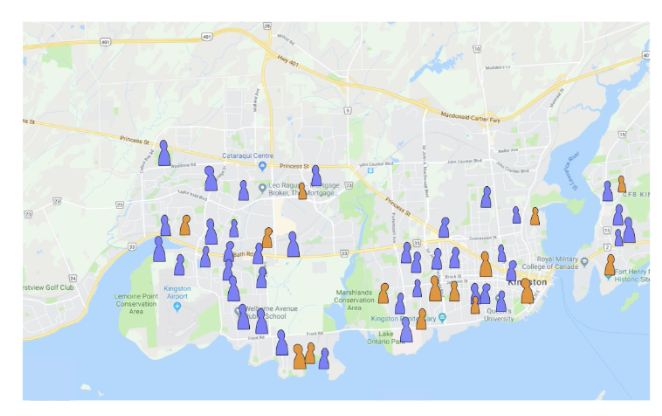
What is this study an example of?
Simple random survey: The sampling unit is selected at random from the statistical population.
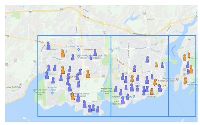
What is this study an example of?
Stratified survey: sampling units are selected from within predefined groups
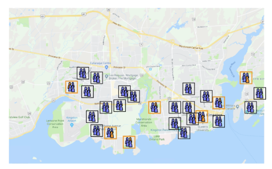
What is this study an example of?
Cluster survey: Groups of observation units are selected at random.
What is the difference between case control and cohort surveys
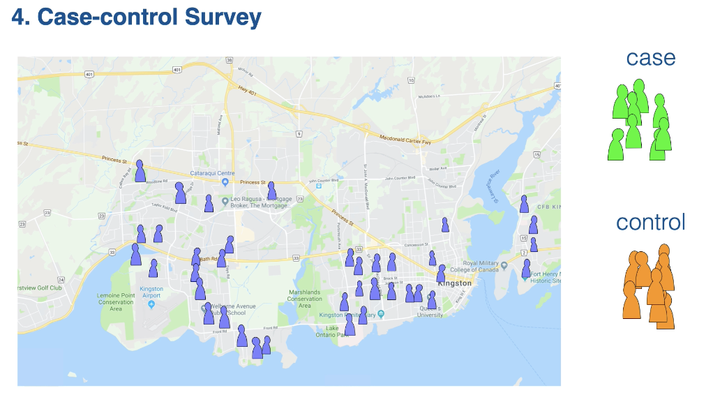
Case-control survey: sampling units are selected based on the response variable. Survey design where the statistical population is divided into a case and a control group based on a response variable to study how other factors might be associated with the observed response.
Collecting two groups
Case: The group with the observed response(outcome)
Control: The group without the observed responses (without outcome)
note other than outcome → each group is the same
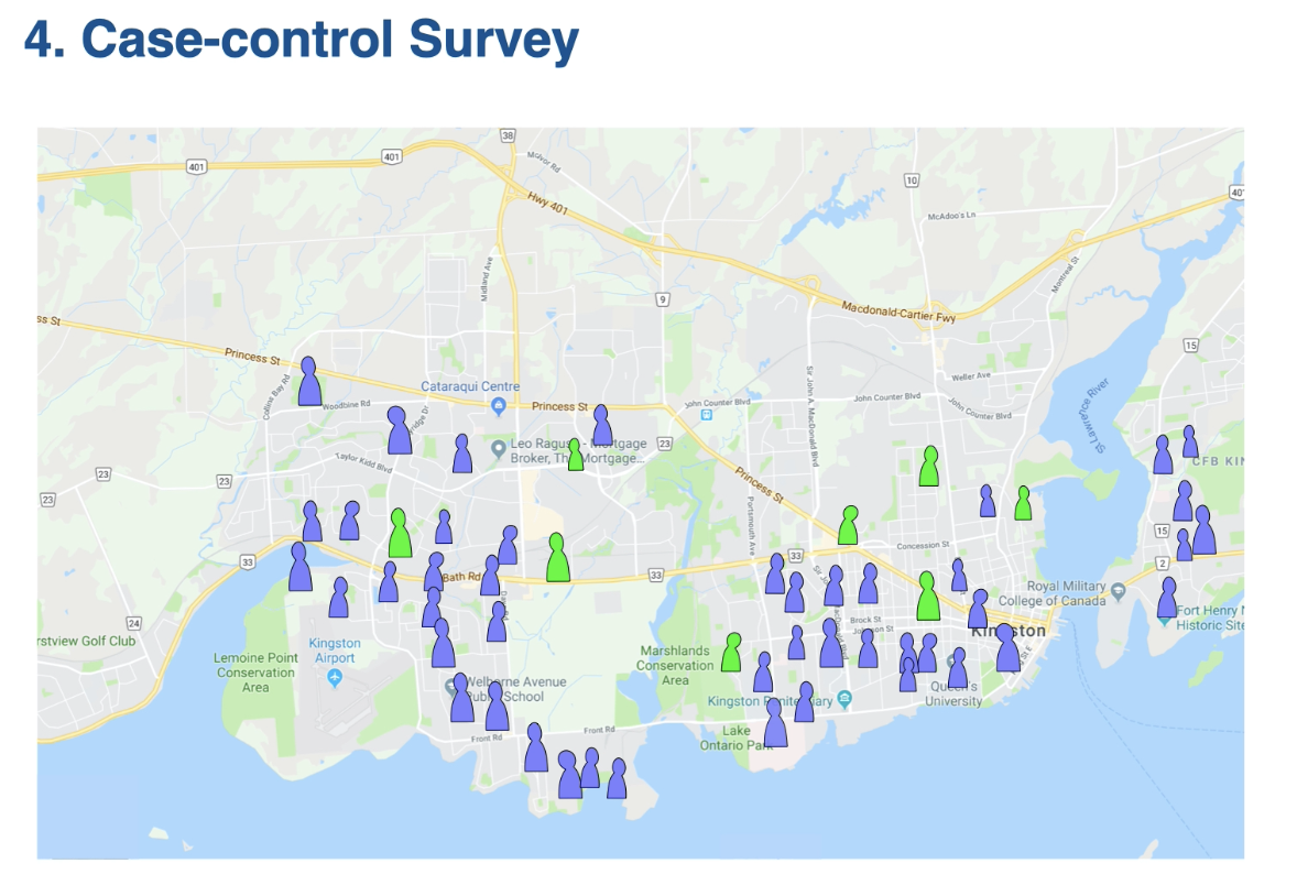
Orange(control): a randomly drawn subset of people who are NOT self-employed.
The key feature of case-control surveys is that the outcome( the response variable) is known and you’re selecting a group that has the outcome and then selecting a comparison group that doesn’t have the outcome to look and see if there are differences in other things between the two groups.
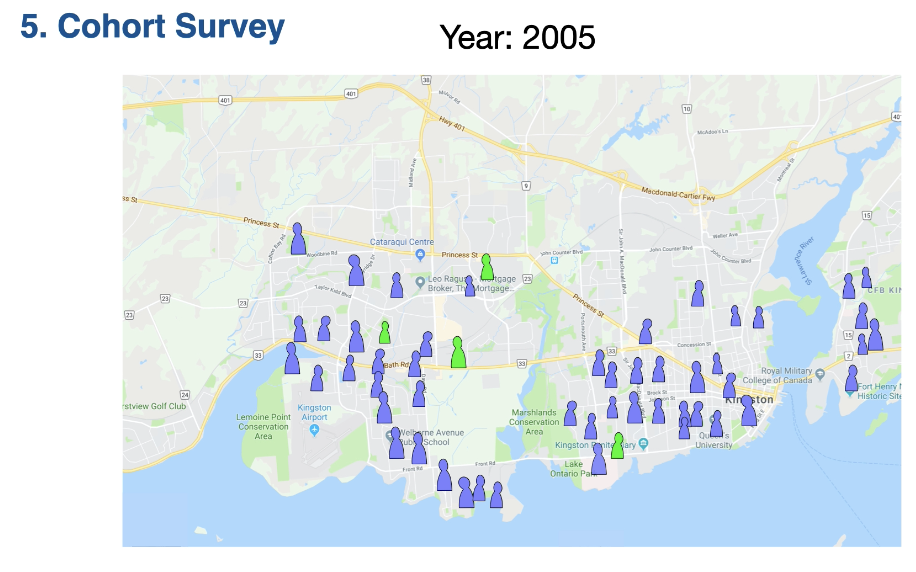
Cohort survey: Sampling units are selected and then followed through time. A survey design where sampling units are selected at random from the statistical population and then followed over time, looking for change in the response variable
We select our sampling units to create a sample and then follow these sampling units through time. This is to see if they develop the outcome that we are interested in.
Ie sampling unit: people that just graduated high school (2005). Follow them through time(2005-2020.. etc) and see if they become self-employed.
Retrospective versus Prospective - This strategy can be used to classify a study. What is the difference between Retrospective and Prospective?
Retrospective studies(looking back in time) are ones where the outcome is already known, which comes with an increased risk of spurious relationships if you are selecting groups based on the outcome. Ie Case-control studies are a good example of a retrospective study.
Prospective studies(looking forward in time) are ones where the outcome is not yet known. These are typically more effort because you need to follow the sampling units for a period of time, but these studies suffer less from spurious relationships. Ie Cohort studies are a good example of a prospective study.
Cross-sectional versus Longitudinal - This strategy can be used to classify a study. What is the difference between Cross-sectional and Longitudinal?
Cross-sectional studies are ones that study a response variable at only a single snapshot in time. ie, consider a study looking at the efficacy of the flu vaccine. A simple random survey of vaccinated people in Ontario measures the amount of the flu virus in blood samples from each sampling unit. Since the measurements were done only at one time, it is a cross-sectional study.
Longitudinal surveys are ones that study a response variable at multiple points in time. Ie Consider again a study looking at the efficacy of the flu vaccine. If you wanted to see whether vaccination maintained its effectiveness over the entire flu season, you could collect blood samples each month from the people in your sample and measure changes over time.
There are two key things that distinguish experimental studies from observational studies. what are these two key things?
In Experimental studies
the explanatory variable is manipulated by the researcher
sampling units are randomly assigned to each level in each factor. As a result, there are two steps where sampling units are selected at random in experimental studies.
Selecting sampling units to ensure that they are an independent and unbiased subset of the statistical population.
Randomly assign the selected sampling units for different treatments within the study.
In the real world, both steps can be done at once; however, for the purpose of distinguishing experimental studies from observational studies, it is helpful to separate each step.
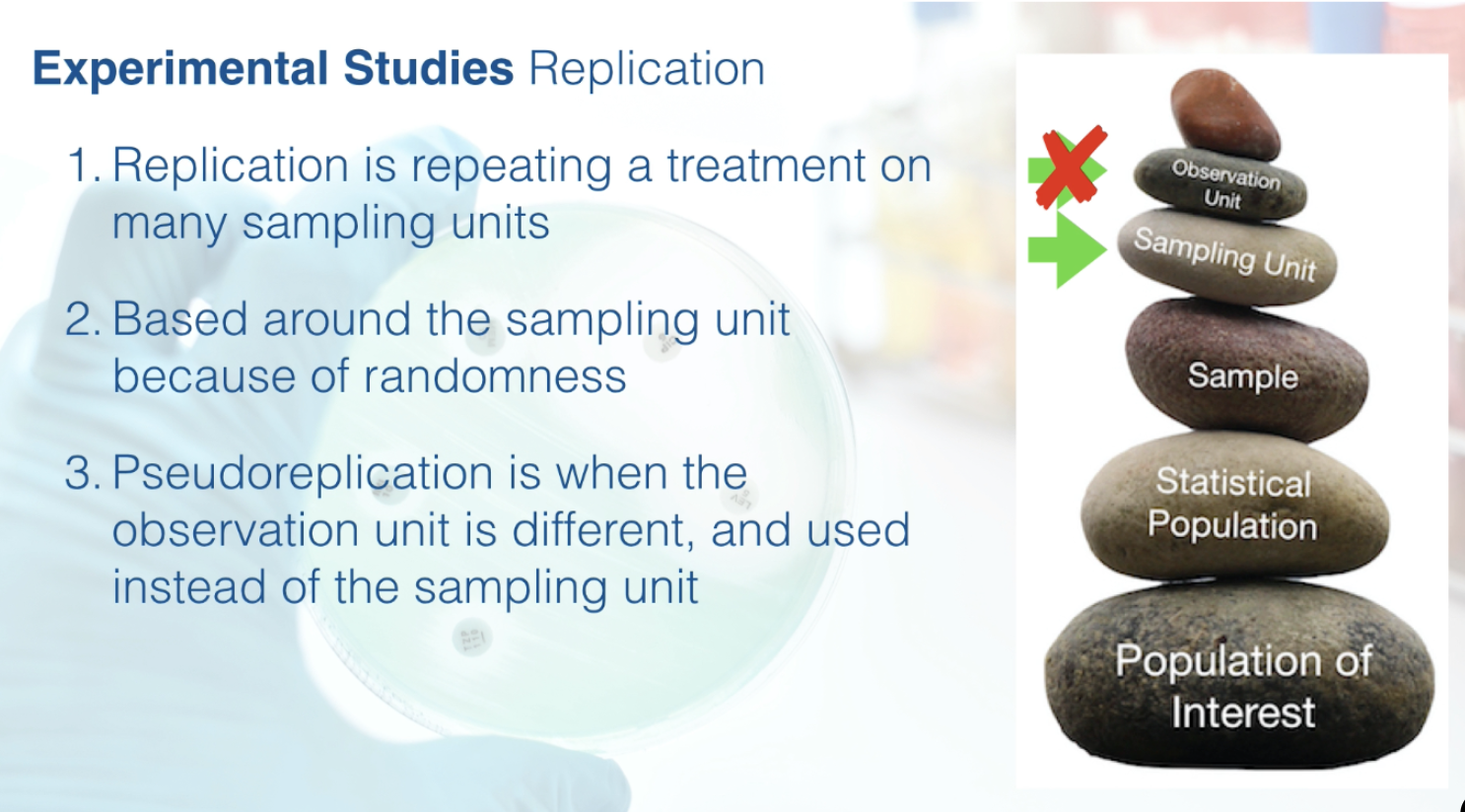
Replication is the corner stone of experimental studies what is the difference between replicates and psudoreplicates?
Replication: it is the idea that a treatment will be repeated a number of times to see how repeatable a measured outcome is. Specifically, replication is the number of times a treatment is repeated on independent, representative and randomly selected units. Ie in statistics is it the sampling unit, and furthermore the replicates are the number of sampling units in an experimental study.
Pseudoreplication:An error created when the units used in an experimental study are not the proper sampling unit and thus are not independent, represetaive or unbiased. Typically it is an error in the design of an experimental study where the observation units are analyzed rather than the sampling units.
What are the 5 ways experimental studies replicate samples
CT. B.B.P.S. = Acronym for the 5 ways
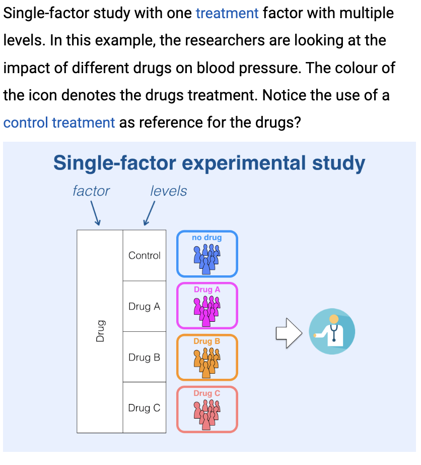
Control treatment: contains everything except the treatment. Is common in experimental studies and is intended as a reference treatment to compare against the treatment levels that alter the explanatory variable. It contains everything that the treatment levels do, except the treatment itself.
Blocking: are predifined groups where treatments are applied within each group. is analogous to stratified sampling, but for experimental studies. It is used to control for variation among the sampling units that is not of interest to the researcher.
Blinded: method that masks the treatment drom the sampling unit(single blind) and researcher(double blind). is commonly used in experimental studies involving people and refers to a design where the sampling unit (usually a person, but could be a group of people) does not know what treatment they are being exposed to. In a single blind design, the sampling unit does not know the treatment they are assigned to. In a double blind design, both the researcher and sampling unit do not know what treatment they are assigned to. The primary benefit of a blinded design is to remove accidental bias caused from the sampling unit or the researcher knowing what treatment is being applied.
Placebo: a substance or treatment with no effect used to create a control treatment. is a method often used in medical trials for the control treatment that helps accomplish a blinded design. It is a substance, or treatment, that has no effect on the response variable.
Sham treatment: a method that is used to create controls for treatments that require handing the sampling unit. is similar to placebo in that it is a method used in control treatments. However, the purpose of a sham treatment is slightly different in that it aims to account for the effect of delivery of a treatment that is not of interest to the researcher.
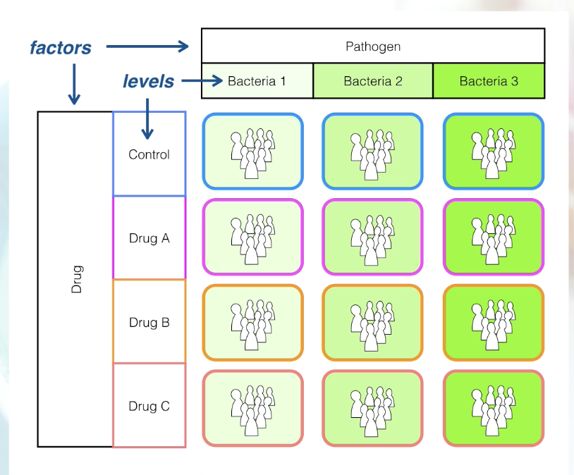
What is the Terminology behind factors and levels as Experimental study labels?
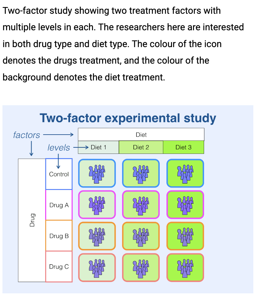
Factors – The type of explanatory variable we are using (i.e. treatment type/drug and pathogen)
Levels – levels are the different values within that factor(i.e. levels of drug... Control, drug A, drug B etc.)
What is the difference between single and two factor experimental studies?
Explain the difference between data vs variables:
Types of Data: Variables vs. Data
Variables - something that is observable from an observation unit
Data(plural) - are the particular values that a variable takes on, from each observation unit
What is the difference between nominal categorical and ordinal categorical? What is the difference between continous numerical and discrete numerical?
The first level of distinction of variables(2):
Categorical variables: vaules that are qualitative. Ie colour or shape
Nominal categorical: NO inherent order of qualitative values(ie colour or political party you voted for)
Ordinal categorical: Inherent order to the qualitative values.(i.e. a scale of values such as “low income”, “middle income”, “high income”.
Numerical variables: values that are numerical. ie numbers
Continuous numerical: value is any non-integer number( ie something like length or height that is 2.356 m)
Discrete numerical: value that is an integer(whole #) count(i.e. the number of patients that entered the clinic on a certain day could be 5 one day and 15 another) discrete numbers vary.
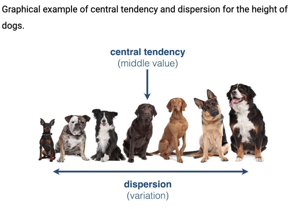
What is central tendency vs dispersion tendency?
Central Tendency: describes the typical value in your sample (e.g., mean)
Dispersion Tendancy: describes the spread of the values (e.g., variance).
How do you calculate the central tendency for numerical and categorical variables including mean, median, counts, and proportions?
Categorical variables:
Categorical data is characterized using counts and proportions. When writing a report, you always want to include the counts in a table, but for descriptive statistics it is often easier to understand the data as proportions.
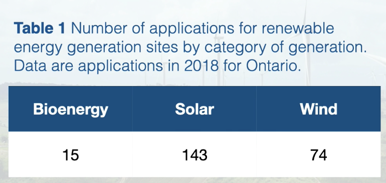
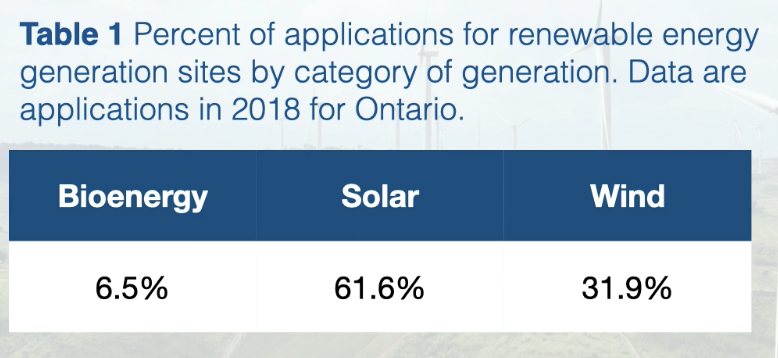
Counts: are used for categorical variables and are the number of observations in your sample that fall into each category.(i.e. in the table below the counts are the number of applications for each bioenergy, solar and wind)
Proportions: are used for categorical variables and are the share of observations in your sample that fall into each category. To get proportions you use counts and turn that data into a percentage. Proportions use percentages rather than just tallies. (i.e. in the example below using tallies allows us to see that solar generation is roughly two-thirds of the power generation, wind one-third, and a very scarce proportion are bioenergy.
* important when you use proportions(percentages) you need to tell people/ at some point display how many counts you had in each category.
Central Tendency & Dispersion
Countsand proportions indicate the central tendencyof categorical data.On the other hand, rangeis used to indicatedispersion, which describes the variation in the response variable(i.e. the proportions above ranges from 6.5%-61.6%)
Numerical Variables
2 different approaches we can use:
..
Numerical Variables Using Means
Numerical data:
Descriptive statistics using means:
Mean describes the central tendency(middle sample)
Variance(and/or standard deviation) describes dispersion
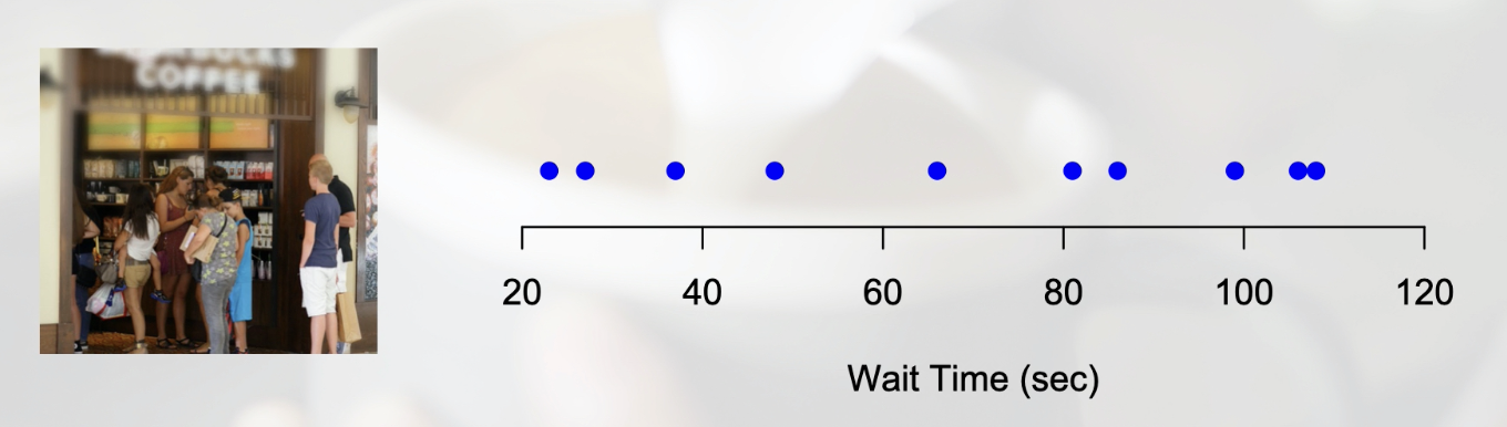
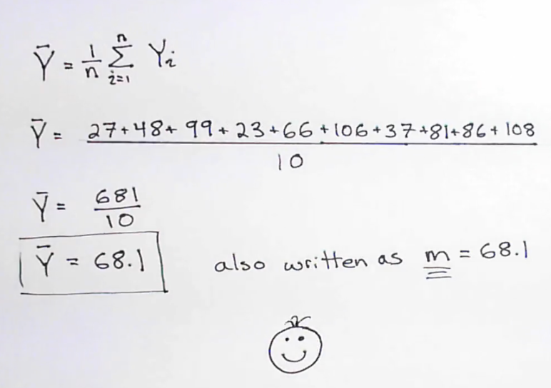
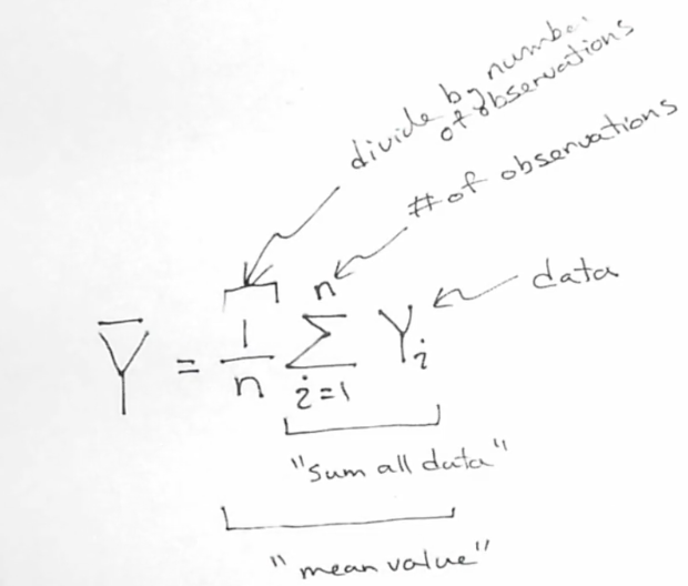
Calculate the mean in two steps:
Sum of all the values in your sample
Dividing by the number of data points(observations) in your sample.
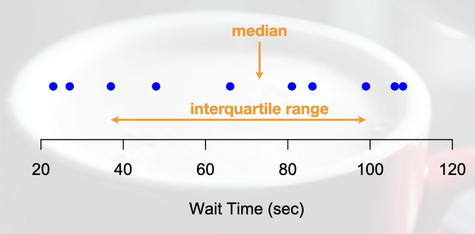
Above blue dots=data points
Use the formula below to calculate the Mean:
above depicts mean of wait time example
How do you calculate dispersion for numerical variables including variance, standard deviation, interquartile range, and range?
Calculations Wait time example: Mean: 68.1 secs, Variance & Standard Deviation: The horizontal line going from 32 secs to 108 secs (horizontal line made from one standard deviation higher than the mean, and one standard deviation lower than the mean)
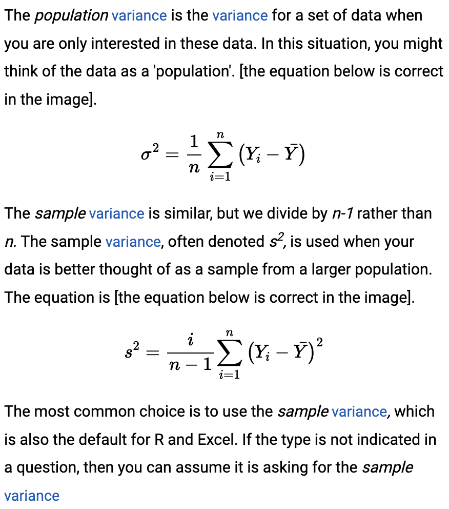
Population vs Sample Variance
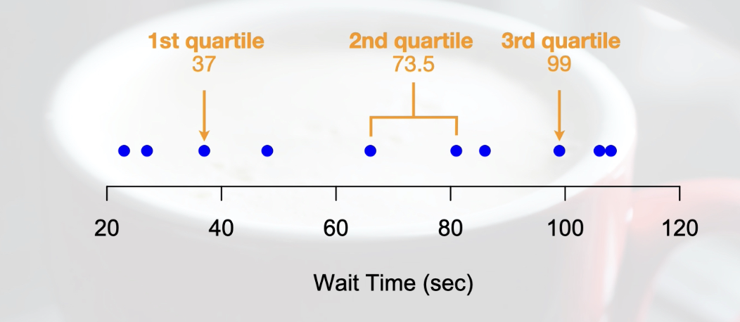
Numerical data: descriptive Statistics using quartiles
Quartiles are ranked bins of your data - take the data set, sort it and then split it into 4 pieces(quartiles). Quartiles let us determine a measure of central tendency and dispersion
Calculating/ finding quartiles:
Sort your data from lowest to highest values
Find the 2nd quartile by splitting data in half according to # of data points(obsv):
If odd: then 2nd quartile is the middle value
If even: then 2nd quartile is the average of two middle values
Find the 1st quartile by creating a subset of the lower-valued half(50% of lower-value observations) of the data set. Then use the rules in step 2 to find the middle value within this subset. **The 2nd quartile is ONLY included in the subset if the total number of observations is ODD. If the 2nd quartile is even, the 2nd quartile is NOT included and the dataset it split between two middle vaules.
Find the 3rd quartile by repeating step 3 by creating another subset but this time for the upper-valued half of the observations. **Again the 2nd quartile is ONLY included in the subset if the total number of observations is ODD. If the 2nd quartile is even 2nd quartile is NOT included, but number in subset that made average are.
Central Tendency & Dispersion:
Central Tendency(middle of data set): describes 2nd quartile, called the median
Dispersion(variation of data): describes the range of the innermost 50% of data, values that the central 50% of data lie over(1st-3rd=?). This difference between the 3rd quartile and the 1st quartile is called the interquartile range(IQR).
Diffences between Quartiles and Means and what makes them better for diffent things?
Pros and Cons of Each: Quartiles vs Means
small datasets → use means
data sets with outliers → use quartiles
Quartiles: Effect on Median and IQR
Pros | Cons |
|
|
Means: Effect on Mean & Standard Deviation
Pros | Cons |
|
|
What is effect size mean?
Effect size: the change in the mean value of the response variable(maniputated variable) among 2 groups. (i.e. the effect size could be the difference between the cost of Starbucks and Tim Hortons coffee if the response variable is the amount of money people are paying for their coffee)
Explain the difference between using a simple difference versus a ratio to quantify absolute effect size
Absolute(difference) and Relative(ratio) Effect Size:
Used to evaluate whether the change in response variable in groups is meaningful
Effect size(for descriptive stats): description of the change in mean among the samples you collected from different groups. this is calculated as a difference or ratio
Difference(absolute): difference in means of two groups; mean of Y1 subtracted by the mean of Y2 (the difference uses the same units as OG means - good to use for length, money, weight, speed etc)
Ratio(relative): proportional change in means of two groups; mean of Y1 divided by the mean of Y2 (good when you are using a scale that you are not familiar with/ meaning not obvious - ie looking at medical studies with percentages of risk for cancer; ratio allows you to understand relative change with inherent meaning)
Differnce between effect size in an Observational study instead of an Experimental study and vice versa?
Observational Studies: effect size is calculated as the change among groups (ie in a case-control study effect size would be the change in the mean value of the response variable between case and control groups.)
Experimental Studies: effect size is calculated among treatment levels (ie in single factor experiment effect size would be the change in the mean value of the response variable(variable being manipulated) among the levels of the factor.
What are contingency tables? what are they used for?
Contingency Tables: are tables of data frequencies or proportions within different levels of categorical variables. (ie surveys to collect data include selecting number of stars)
Difference between conditional distribution and marginal distribution? What can each of them help us find in our data? when looking at contingency tables
Conditional distribution: are two-way tables that show the proportion of sampling units for one variable within each level of the second variable.
Conditional Distributions: visualize potential for relationship between columns and rows
Help Visualize interactions between variables(in a way marginal distributions cannot)
Different because conditional distributions: looking at the relative proportion of the sampling units across the levels of one variable but within just a single level of the other variable
Looking for relative abundance in single collum (finding proportions within single collum)
Marginal distribution: are the row and column sums of a two-way contingency table. They can be shown as frequencies or proportions.
Marginal distributions: overall patterns of sampling units across both columns and rows
Magenial distributions can help us see patterns in our data that may otherwise be hard(we can figure out if the 6 sampling units that have 2 cats or dogs are a small number or a big number).
Magenial distributions are tallies/sums of data collected in the rows and the columns, marginail distributions can be shown as counts or proportions
Difference between one -way and two way contingency tables?
One-way and Two-way contingency tables
One-way and two-way contingency tables rely on the number of categorical questions you ask of your sampling unit.
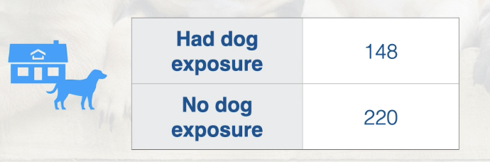
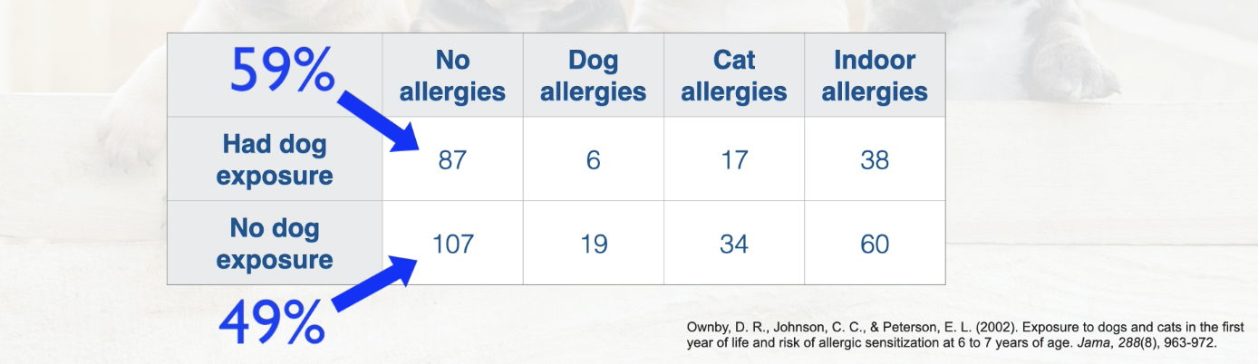
The case study (used to explain): does having dogs as childl prevent you from having allergies as an adult?
One-Way Contingency Table: only ONE categorical variable per single sampling unit
Ie to formulate the table above question was asked: “Did you grow up with dogs?” so this is a one-way contingency table - because it asked one categorical question of a single sampling unit.
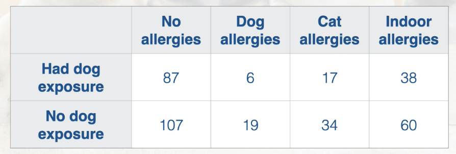
Two-Way Contingency Table: TWO categorical variables per single sampling unit
1st categorical variables should be the focus of the study
2nd categorical variable will then be the additional categorical variable
Ie to formulate the table above question was asked: “Did you grow up with dogs?” AND “Do you have allergies?” this is a two-way contingency table - because it asked TWO categorical questions of each single sampling unit.
1st categorical variable: is allergies, this is because the study is about provenance of allergies
2nd categorical variable: dog exposure
Results from this study showed that being exposed to a dog as a kid reduced chances you would have allergies as an adult.
When should you use a bar graph? what type of data is good for being displayed on a bar graph? what is the one case that bar graphs can be used for numerical data?
Bar graphs are best used to:
Visualize categorical data
Can be used alongside contingency tables
They can be used for single and two-variable categorical data but should NOT be used for numerical data
Case when bar graphs can be used for numerical data:
Statistical datasets have categorical information on many sampling units. But people often collect data that characterize a system that are not statistical in nature. For example, if you wanted to characterize the amount of renewable energy generated for each province in Canada, then you would have data where each province (categorical) has a single numerical value (amount of renewable energy). This type of data is often depicted by a bar graph, which is fine. However, it's important to keep in mind that the data are not statistical in nature because they don't represent a subsample from a larger statistical population.
**if one varible is numerical and the other is categorical use box plots NOT bar graphs
When should you use a histogram? what type of data is good for being displayed as a histogram? what is a bin?
Histogram: figure used to visualize numerical data the vase of the graph is the numerical variable that is divided into a number of bins. The graph is then created by plotting the number of sampling units(frequency) in each bin.
For numerical data(can easily be mixed up with bar graphs but are notttt the same)
No gaps to represent continuum because numerical
Bin: is a small range of the numerical variable. The numerical variable is divided into a number of bins of equal size forming the base of the figure.
Disadvantages: **if one variable is numerical and the other is categorical use box plots NOT histograms
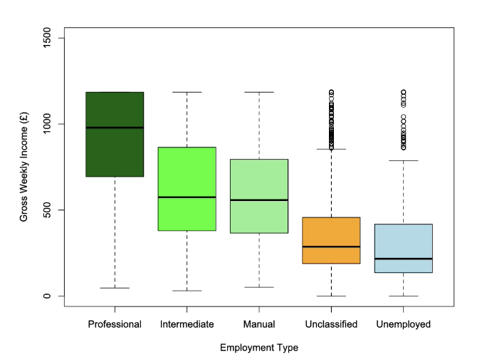
When should you use a box plot? what type of data is good for being displayed on a box plot?
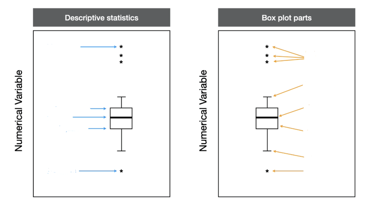
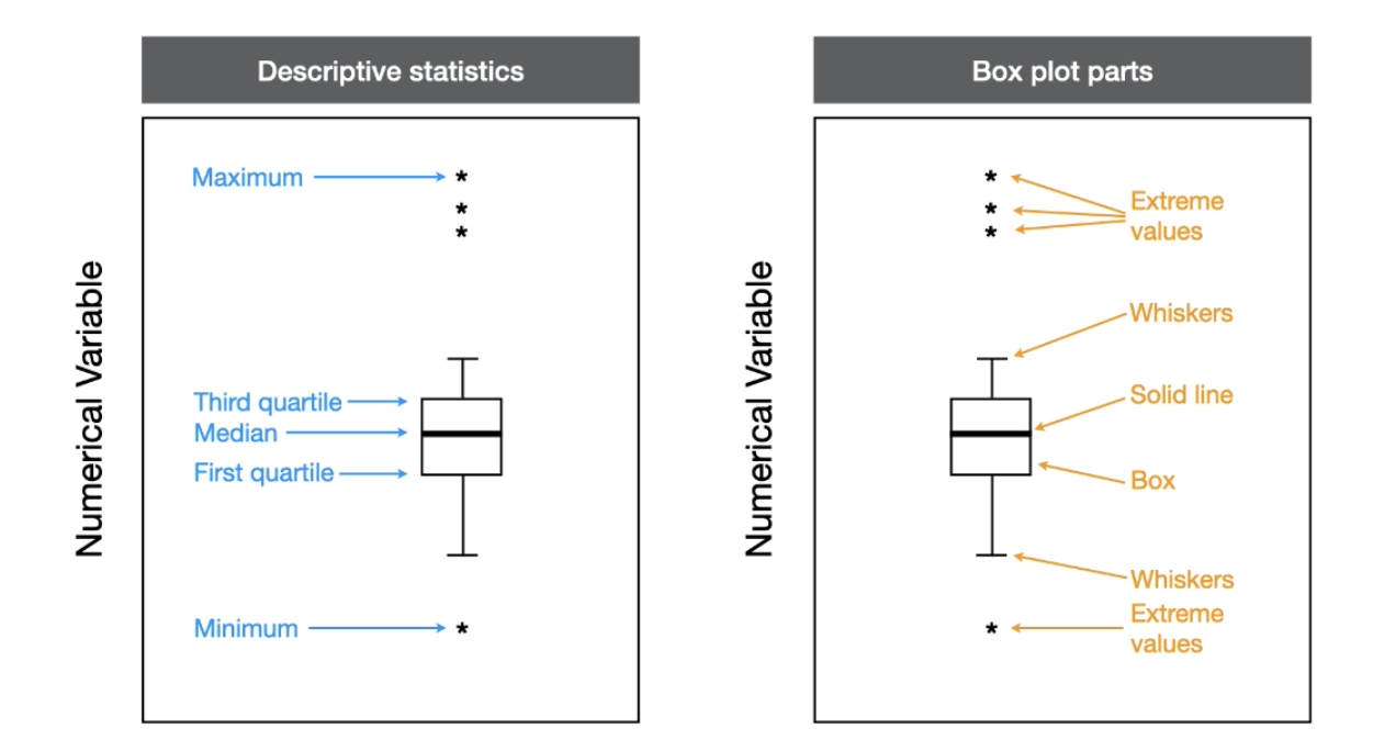
Box plots:
Mainly used for numerical data but can be used if their is a combination of numerical and categorical data
Based on quartiles
Show five descriptive statistics: min, first quartile, median, third quartile, and max
…full name: box and whisker plots LOL
Anatomy of a boxplot…
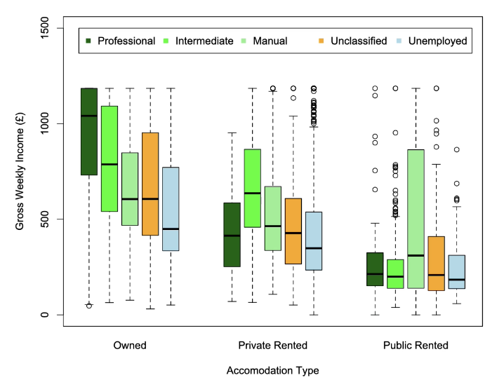
Group plots, 1 catagorical group s 2 catagorical groups
1 categorical group
Box plots vs histograms pros and cons of each
Histograms
Pro | Con |
The main advantage of histograms is that can be used to illustrate the shape of the distribution. | The main disadvantage is that it is difficult to look at a numerical variable across categorical groups. |
Box Plots
Pro | Con |
The advantage of box plots are that it is easy to compare across multiple categorical groups. | Box plots convey much less about the shape of the distribution in a sample. |
When should you use a scatter plots? what type of data is good for being displayed on a scatter plots?
Scatter Plots:
Two numerical varibles you want to compair coming both variables coming from individual sampling units(asked two questions/ know two things about one sampling unit)
Each point is a sampling unit
The horizontail is the x-axis and the vertical is the y-axis
When should you use a line plots? what type of data is good for being displayed on a line plots?
Two numerical variables: measured repeatedly from the same sampling unit
one sampling unti line plot vs mutiple sampling unit line plot
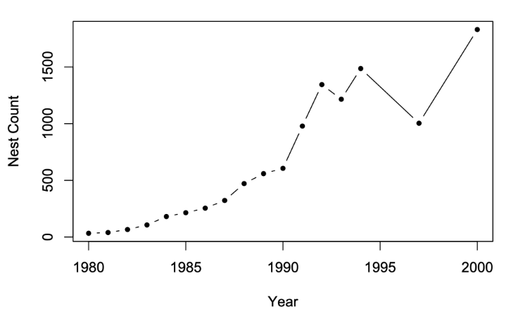
‘Typical’ one sampling unit on line plot:
Circles - represent a repeated measure of the same colony
Line - represents a trend in population size for the colony
Overall line plot - sampling unit
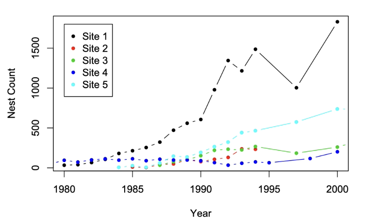
Mutiple sampling units on one Line plot:
Each site is a sampling unit^
covariate is a name, who/ what is this name given to?
covariate is the name given to the x-axis and y-axis when i) the data showcase descriptive statistics and are from an experimental study, or ii) the data are showcasing inferential statistics and the statistical test is about association.
What is the differnce between the predictor varaible and the reposnse variable when graphing
Predictor Variable: is the name given to the x-axis when the data are showcasing inferential statistics and the statistical test is about prediction.
Response variable: is the name given to the y-axis when the data are showcasing inferential statistics and the statistical test is about prediction.
What is a random trial? how is randomness connected to collecting samples?
Random trial: Any process with multiple outcomes but where the outcome (result) on any particular trial is unknown. (ie with a coin, it could be head or tail but on each trial the outcome of a head or tail is unknown)
Connecting randomness to sampling: Selecting a sampling unit is considered a random trial
The act of taking an observation on a sampling unit is considered a random trial. This is because we don’t know what the outcome is going to be when we select the sampling unit
What is the differnce between a sample space and an event?
Sample space: The list (set) of all possible outcomes from a random trial, ie for the trial flipping a coin the sample space is S={heads, tails}.
Event: is the outcome of interest. Whochi is a subset of sample space ie the event if we are interested in the probability of getting a head when flipping a coin our event is E={heads}.
Difference between discrete and continuous variables?
Discrete variables: represent counts (e.g. the number of objects in a collection).
Continuous variables: represent measurable amounts (e.g. water volume or weight)
What is probability? and how does the law of large numbers help define probabilities?
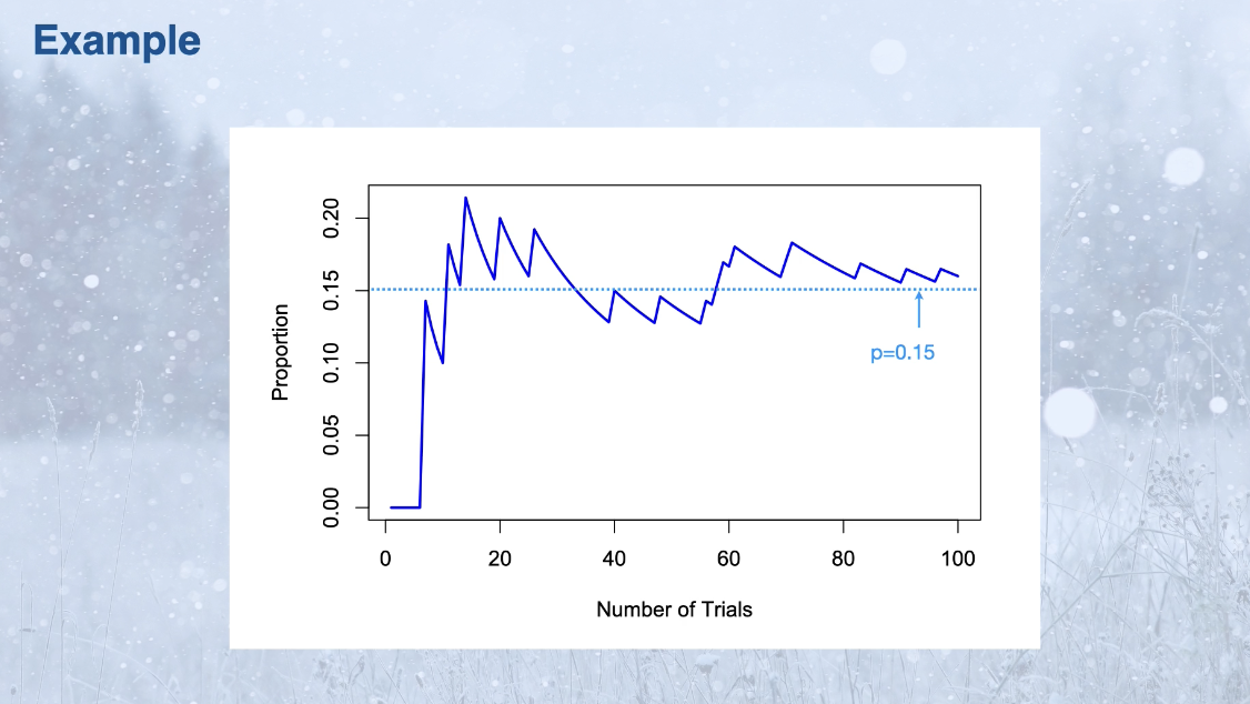
Probability is the proportion of time that an event would occur if the random trial were repeated many times
Law of large numbers - probability is the proportion of time we see an event over manu many repeated trials.
Sometimes we can calculate the probability of we can simulate the random trial(simulating doesn’t change the probability that already exists)
A probability distribution has two types: contious and discrete, what difference variables do each of them consider?
Probability distribution: Functions that describe probability over a range of events.
Looking at a range of events
Functions that describe the probability of many events
The probability of overseeing an outcome within a range of events is the area under the function(curve).
Continuous probability distributions: Probability distribution for a continuous variable
Discrete probability distributions: Probability distribution for a discrete variable
Main distinction between discrete and continuous distributions
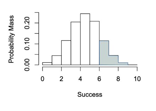
Discrete probability distributions:
Probability distribution for discrete numerical random variables. Ie flipping a coin and want to know the probability of getting a head out of 10 flips, that would be a discrete random variable and therefore a discrete probability distribution.
Typically shown as vertical bars with no space between events(similar to histogram)
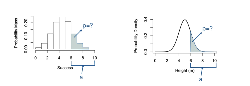
The Y-axis is the probability mass
For example, if we were to look at flipping the coin to get a head 6 or more times our probability is shown in grey.
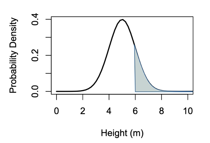
Continuous probability distributions:
The probability distribution for continuous numerical variables.
Show as a single curve across a continuous event
Probability of a single event in a continuous distribution is always zero
The Y-axis is the probability density
For example, characterizing the distribution of tree heights in a forest height is a continuous numerical variable hence the x-axis that can be shown using continuous distribution.
Still looking at the area under the curve so if we wanted to know the probability that a randomly selected tree was 6m or taller the probability would be shown in grey.
you can calculate a probability from a range and probabilities from a standard normal distribution, how is this done?
Calculate probabilities when we are given a range
First, select a range (in the example below a=range selected)
Calculate the area that is under the curve for the range (in the example below p=probability)
Most often you must use a computer - prase yee the lord
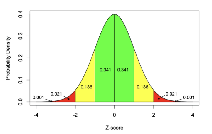
Standard Normal Distribution:
Used to answer any question that is based on probabilities from a normal distribution. This is done by converting the original question into a standardized form.
A special case of the normal distribution with a mean of zero and a standard deviation of one.
Makes the calculator of probabilities more straightforward
This example is a continuous distribution.
Each step on the z-axis represents one standard deviation
Ie from z-score from 0-1 the probability is 0.341 etc.
Any problem that’s based on normal distribution can be converted into standard normal form which makes the calculations quite straightforward.
How to do conversion from normal form→ standard normal form:
Explain the difference between calcualting ranges and probabilities
Ranges vs Probabilities:
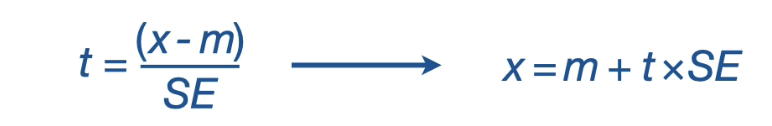
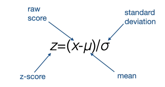
Calculating Probabilities The mean (μ), standard deviation (σ) and value of interest (x) in a problem are used to calculate a corresponding z-score from the equation z=(x-μ)/σ. The z-score is then used to calculate the probability over a range from the standard Normal distribution
Calculating Ranges The probability and range description in a problem are used to calculate a z-score(z) from the standard Normal distribution. Along with the mean (μ) and standard deviation (σ) in the problem, the z-score(z) is then used to calculate the value of interest (x) from the equation x=μ+zσ. The calculated x is the value of interest on the non-standardized scale and defines one side of the range. The other side of the range typically is the positive or negative extreme (i.e., +/- infinity).
What are population parameters? what are they used to do? What is the key difference between descriptive statistics and population parameters? how is the labelling distinguishably different from descriptive statistics?
Population parameters:
Describe attributes of the statistical population (ABSTRACT CONSTRUCT)
Each measurement variable has its own set of population parameters (ie average cost of rent and on-campus numerical value or on vs off campus categorical value has its own set of population parameters)
Labelled using the Greek alphabet such as: ρ, μ, σ
Population parameter values are considered fixed (meaning that anyone surveying should get the same data and the same results)
Recall descriptive statistics:
Are any quantifiable characteristics of a sample
Each measurement variable has its own set of descriptive statistics
Labelled using the Latin alphabet such as p, m, or s (ie mean = little “m”)
KEY Difference:
The population parameter is fixed: estimated by sample data
This means mu and sigma are fixed.
ie if I go collect the weight of all the chickens or someone else goes to collect all the weight of the chickens the mean will be the same either way
The descriptive statistics will vary each time a new sample is drawn
Ie if I go collect the weight of all chickens or someone else goes to the sample, and graph will vary because not the same sample.
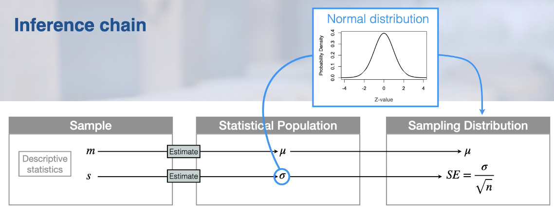
How does an estimation relate descriptive statistics to the population parameter?
Estimation:
Descriptive statistics provide an estimate of the population parameter
The causal(causation) connection between the sample and the statical population is important for building framework for inference
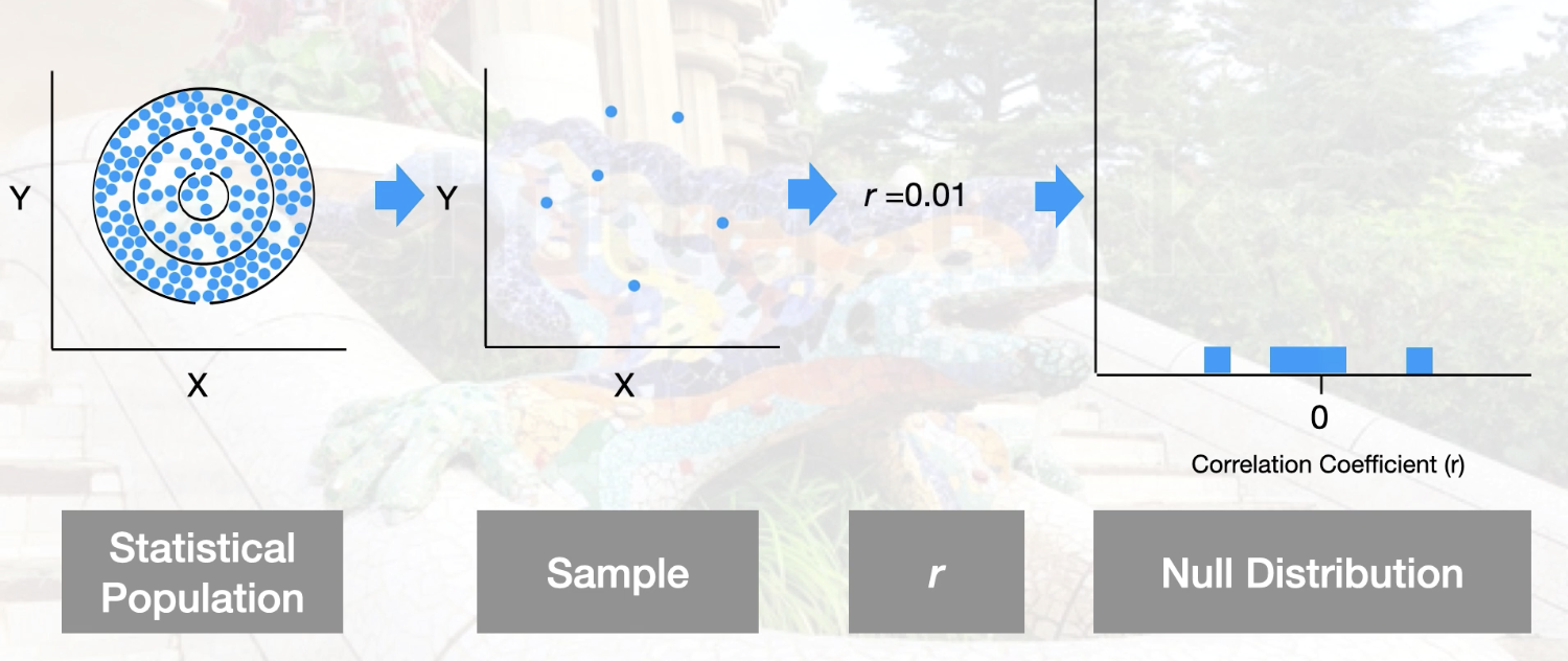
What are sampling distributions?
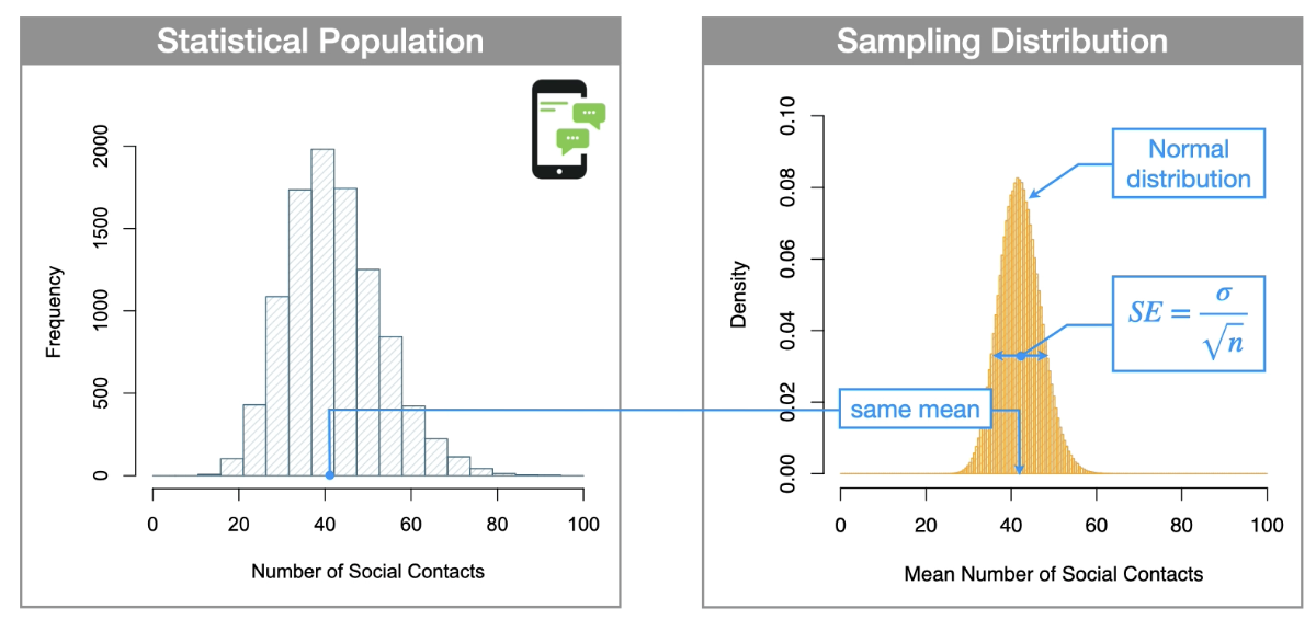
Sampling distributions: is the probability distribution of a descriptive statistic that would emerge if a statistical population was sampled repeatedly a large number of times.
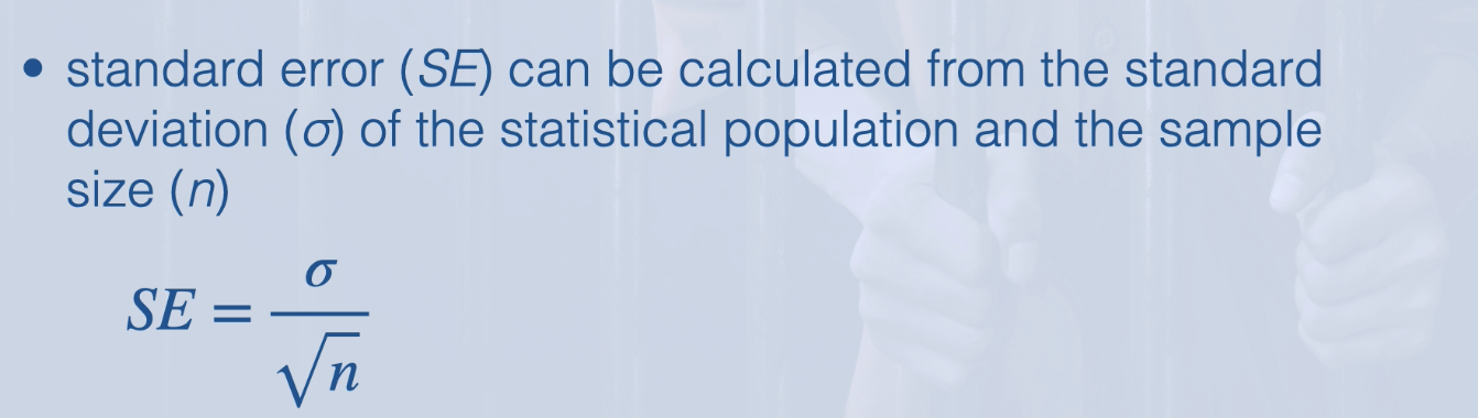
What is standard error and how is standard error calculated?
Standard error:
By definition is the name that is given to the standard deviation of the sampling distribution. (awk cause no mistake/error involved)
Thus the sampling error can also be called the standard deviation of the sampling distribution (and represented as σvector x )
The standard error is very important for making a statistical inference
Standard error will only ever be used to talk about the standard deviation of a sampling distribution.
What are the two key characteristic that central liit theorem tells us that sampling distributions have?
Central Limit Theorem tells us:
Sampling distribution has two key characteristics
Shape independence - the shape of the sampling distribution is independent of the statistical population (as long as your sample size is large enough)
When the sample size is large enough the sample distribution is bell-shaped, even if the population is not
The variance depends on sample size - the variance of your sampling distribution or the standard deviation depends on the size of the sample
low sample = large variance
Is a sampling distribution a normal distribution?
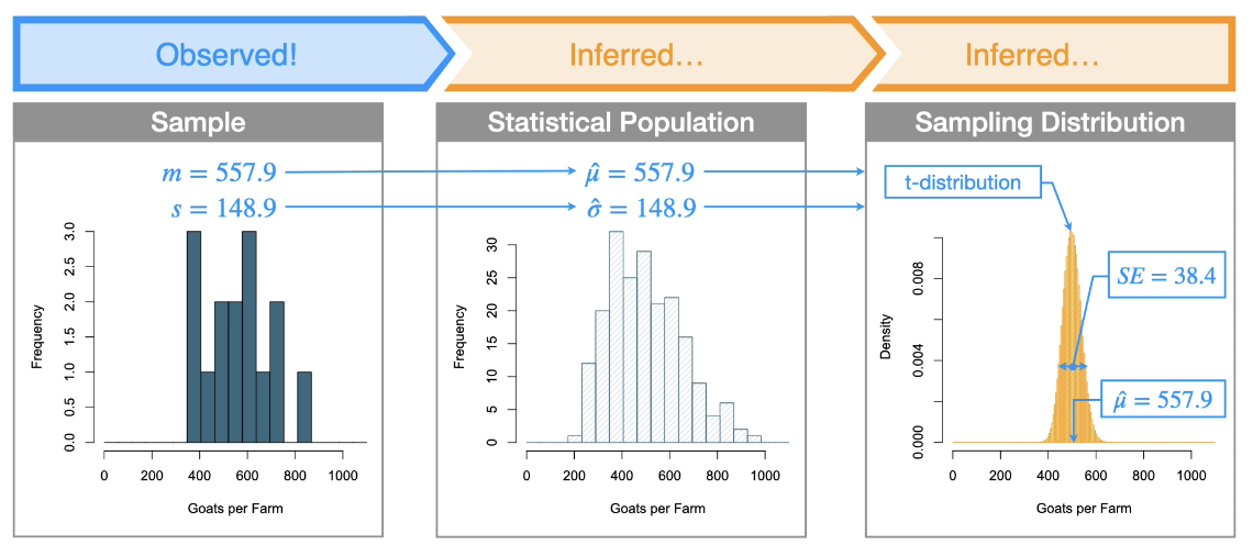
What is “Chain of Interference? what are the 3 steps?
Chain of Interference
The statistical population and sampling distribution are never observed directly
Our sampling distribution is not something that is constructed in practice
The sample is the only thing that is observed directly

Take the observation in our sample
Make an inference about the statistical population in particular its parameters
Then use observation and inference to calculate and estimate the sampling distribution.
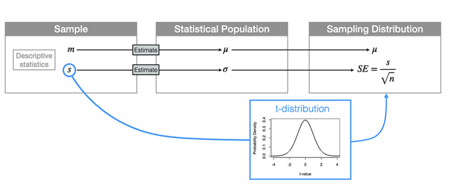
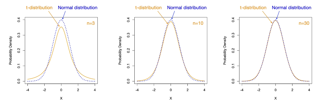
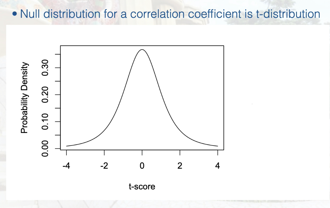
What is a t-distribution? why is it different than the normal distribution? How is the chain of interference altered when using a t-distribution?
The t-distribution:
Looks like a normal distribution
The tail ends are a little bit fatter than a normal distribution and that is to account for the uncertainty of our estimate of sigma
Sample size influences its shape through what is called degrees of freedom which is also a reflection of our certainty in our estimate of sigma
The larger our sample size the better the estimate and the more that the t distribution looks like a normal distribution.
The central limit theorem says that if we know sigma in the statistical population, then our sampling distribution is a normal distribution.
Our problem is that we never know that for certainty we only have an estimate of it.
If we need to estimate that sigma then the final sampling distribution is instead a t-distribution
Example:
From a sample, we are able to infer the key characteristics of the sampling distribution
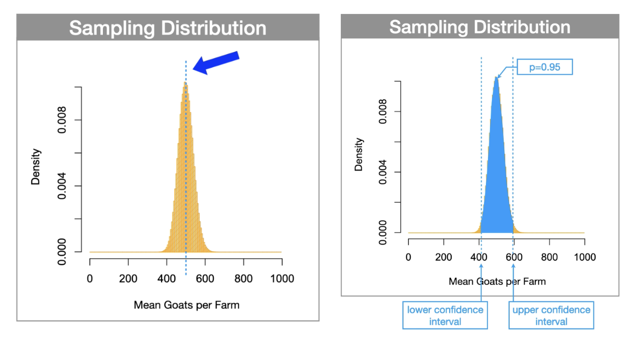
What are confidence intervals? what are they used for?
Confidence intervals: are the range over a sampling distribution that brackets the centre-most probability of interest. (just an ESTIMATE)
Confidence intervals……
Describe the uncertainty in the descriptive statistics of a sample
Derived from sampling distributions
The range over the x-axis of a sampling distribution that brackets; where new samples(values) may be found with some certain probability
Initially, the confidence interval goes in the middle of the distribution (lines sitting ontop of one another). We move these lines slowly away from each other and look at the probability that’s between them. Once we hit the specified probability we are interested in… (typically p=0.95 or 95%) then the location where those two thresholds(brackets lie are our confidence intervals.
how do you calcualte confidence intervals(2 steps)
Steps to Calculate Confidence intervals:
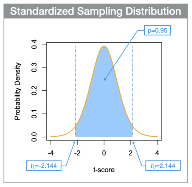
Find the intervals on the standardized scale of the t-distribution.
Using statical software or statical tables: The first step is to use the t-distribution to find the locations on the x-axis that correspond to the probability of interest(these are the left and the right t-cores that bracket the 95% of the probability. These standardized t-scores, which we can label tL and tU to represent the lower and upper confidence intervals on the standardized scale.
Convert to the raw scale.
The second step is the reverse process of the conversion to the standardized form shown above.
The second step is to convert the standardized t-scores back to the raw scale. We will use xL and xU to represent the lower and upper confidence intervals on the raw scale. The raw-scale confidence intervals are calculated as:
xL=m+tL×SE
xU=m+tU×SE
What is hypothesis testing? What is the difference between the Null hypothesis and the alternative hypothesis?
Hypothesis testing: is the process used to evaluate statistical significance.
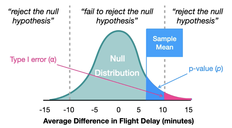
Null hypothesis: is a statement, or position, that is the skeptical viewpoint of your research question. (ie testing difference between flights being delayed between multiple airlines.. And how long flight delays are, the Null hypothesis would be: there is no difference in how long flights are delayed between airlines. And would be written as:
H0: There is no difference on the duration of flight delays between different airlines
Alternative hypothesis: is a statement, or position, that is the positive viewpoint of your research question. (ie in airline delay example the alternative hypothesis would sugges that there is a difference in duration between airlines. And would be written as:
HA: There is a difference in the duration of delays between different airlines.
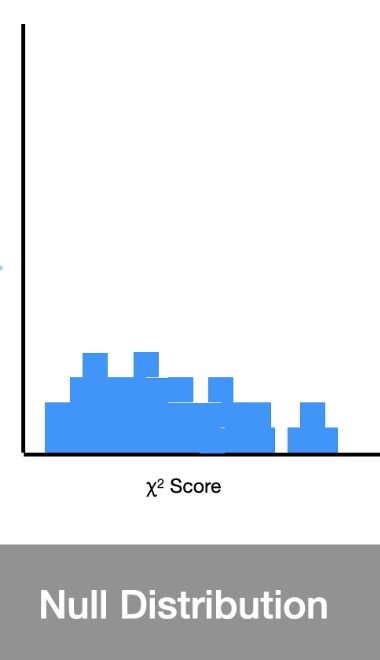
What is the null distribution and when is it used? and what is statisical signifigence and how does it relate to the null hypothesis?
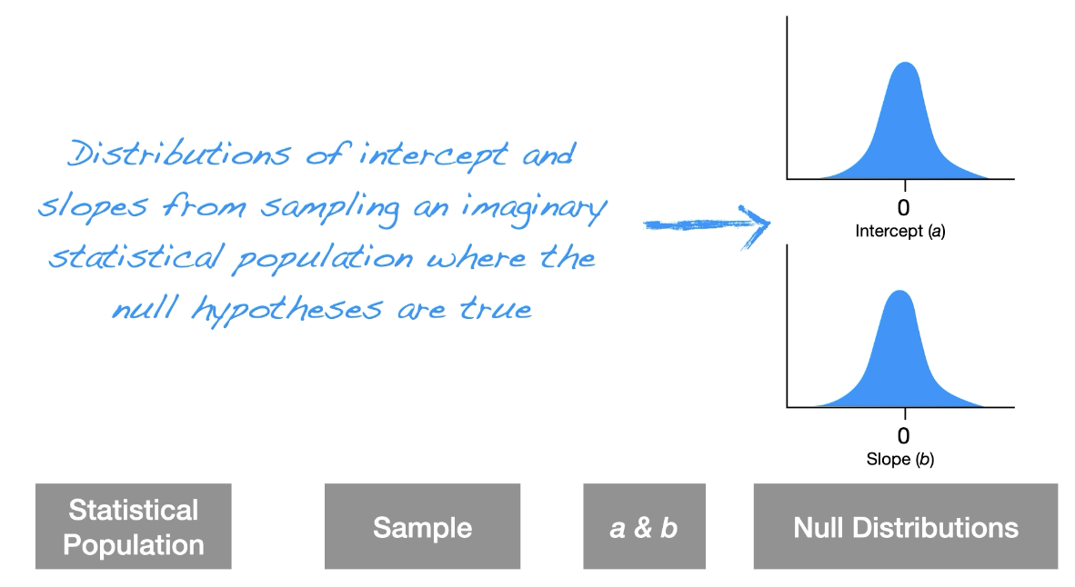
Null distribution: is the sampling distribution from an imaginary statistical population where the null hypothesis is true
Statistical significance: is the conclusion that a set of data are unlikely to come from the null hypothesis.
What are the 4 steps for hypothesis testing?
Define the null and alternative hypothesis
Establish the null distribution
Conduct the statistical test
Draw scientific conclusions
What is crucial when defining your null and alternative hypothesis?
Relationship between Null and Alternative Hypothesis MUST:
Mutually exclusive of each other: meaning the alternative hypothesis contains everything that is NOT in the null hypothesis.
Together must be exhaustive: meaning they must contain all possible outcomes you could have from your study.
Convert statements using symbols whenever possible
This means making symbols for the hypothesis and also symbols for the outcomes. Ie making: TA = flight delay for airline A, TB = flight delay fo airline B. Then the word statements of the null and alternative hypotheses can be rewritten as
H0: TA = TB,
HA: TA ≠ TB
Define if we have directionality in the null and alternative hypotheses in terms of the measurement variable. An example of the test question that would cause directionality would be “Is the delay time for airline A longer than airline B
Directionality in Null and Alternative Hyp: (with airline example)
H0: Airline A has shorter or equal delays compared to Airline B
H0: TA ≤ TB
HA: Airline A has longer delays than Airline B
HA: TA > TB
How do you establish a null distribution?
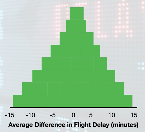
Recall the null distribution is the sampling distribution from the statistical pop where the null hypothesis is proven.
In our example used with flight delay here is what our Null distribution would look like:
How do you conduct a statistical test? What are the rules for making a statistical decision?
Two outcomes are:
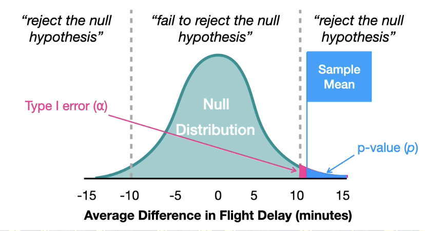
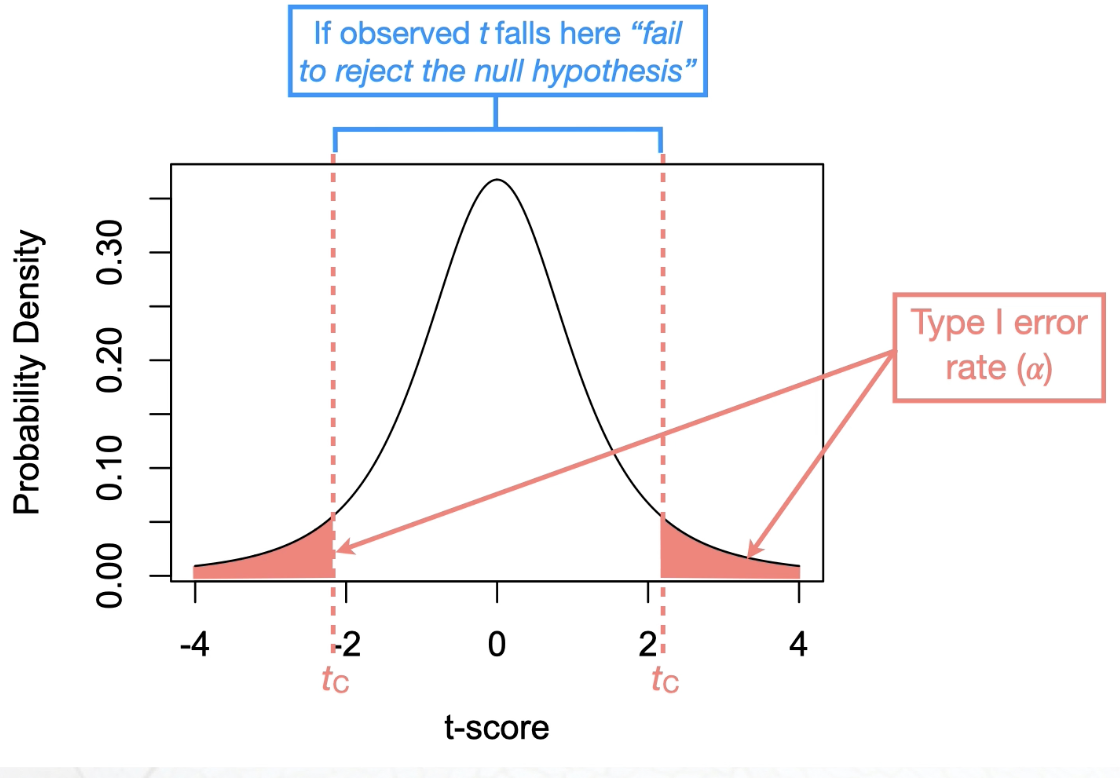
If it is likely that your data could come from the null distribution, then "we fail to reject the null hypothesis."
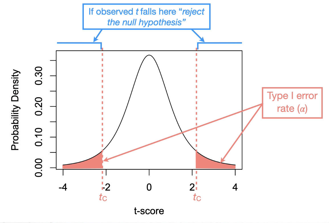
If it is unlikely that your data could come from the null distribution, then "we reject the null hypothesis."
Need two probabilities from the null distribution
the Type I error rate, which is often called alpha (⍺).
The Type I error rate is the probability of rejecting the null hypothesis when it is true.
The second probability is called the p-value (p).
The p-value is the probability of seeing your data, or something more extreme, under the null hypothesis.
Rules for making a statical decision
(p > ⍺)
If the p-value is less than the Type I error rate (p>⍺) then we reject the null hypothesis
(p ≥ ⍺)
If the p-value is greater than or equal to the Type I error rate (p≥⍺), then we fail to reject the null hypothesis.
How do you draw scientific conclusions? What are the two steps for writing your conclusion?
Taking statistical decisions and drawing them back to the research question.
Two Steps:
Strength of inference
If we reject the null hypothesis we could write… “The sample data provide strong evidence that the flight delay is different between airlines”
If we failed to reject rhe null hypothesis we could write…. “The sample data did not provide strong evidence that the flight delay is different between the airlines”
Effect size (only consider when the statical conclusion is to reject the null hypothesis)
We need to connect our statical decision with a scientific context - ie is our sample size large enough to be relevant?
If the effect size was small ( ie wait time is 2min diff), then we might conclude: “There is a statistical difference but it is unlikely to have an impact on consumer choice”
If the effect size is large(ie wait time is 30min diff) then we might conclude: “There is a statical difference that is likely to have a large impact on consumer choice”
What are error rates? What are the two types of error rates used in this Stats course?
An error rate is the probability of making a mistake
Error rates we use:
Type I: is the probability of rejecting the null hypothesis when it is true.
Type II: is the probability of failing to reject the null hypothesis when it is false.
What is the difference between Type I and Type II error rates?
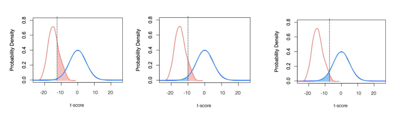
Type I vs Type II error:
Type I error is under the null distribution, whereas the Type II error is under the alternative distribution.
Type I error: is the probability of rejecting the null hypothesis when it is true.
Under null distribution(focus on null distribution)
It is the probability of seeing that data point or something more extreme under the null distribution
For hypothesis testing Type I is known because we can characterize the null
We typically set the Type I error rate as a threshold and then we ask whether the data falls on one side or the other side:
In order to decide if we should fail or reject the null hypothesis
Type II error: is the probability of failing to reject the null hypothesis when it is false.
Under alternative distribution(focus on alternative distribution)
It is the probability of seeing that value or something more extreme under the alternative distribution
We do NOT know anything about the alternative distribution so LOL studying Type II is uncommon. (we still do it tho cause we can gather information from trade-off)
Why do we study Type II if they just an abstract construct?
Why do we even study type II error rates??
While Type II error rates are typically unknown, they tradeoff with the Type I error rate
Since the error rates are under different distributions when one error rate decreases, the other increases.
There are three kinds of t-tests; two sample, paired sample and, single sample, which is which?
"Is the mean standardized test score from a sample of high school students different than the national standard?".
"Comparing exam scores from before versus after tutoring support, did tutoring increase the mean exam scores for a sample of students?"
"Does the mean exam score of a sample of students in a rural high school differ from the mean exam score of a sample of students in an urban high school?"
Single-sample t-tests evaluate whether the mean of your sample is different from some reference value. For example: "Is the mean standardized test score from a sample of high school students different than the national standard?".
Paired-sample t-tests evaluate whether the difference in paired data is different from some reference value. For example: "Comparing exam scores from before versus after tutoring support, did tutoring increase the mean exam scores for a sample of students?"
Two-sample t-tests evaluate whether the means of two groups are different from each other. For example: "Does the mean exam score of a sample of students in a rural high school differ from the mean exam score of a sample of students in an urban high school?"
What is an Expected contingency table? what is it used for?
Expected contingency table: is the contingency table of expected frequencies under the null hypothesis.
Provide a reference to compare the observed data against.
How to calculate expected from ONE way and TWO way observed contingency tables
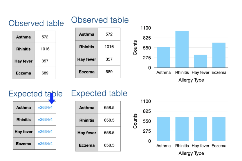
One-way Contingency Tables:
Expectation: Counts are distributed equally among cells
the expected table always given as counts
The sum of all expected counts must be the same as the sum of all observed counts
While the observed contingency table only has integer counts, the expected contingency table typically has a fractional value
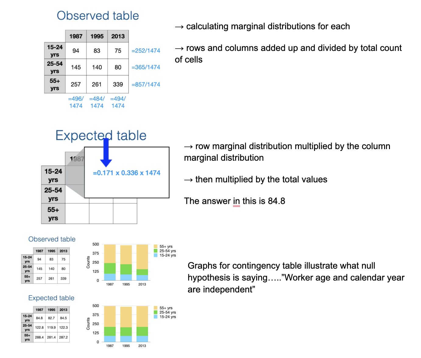
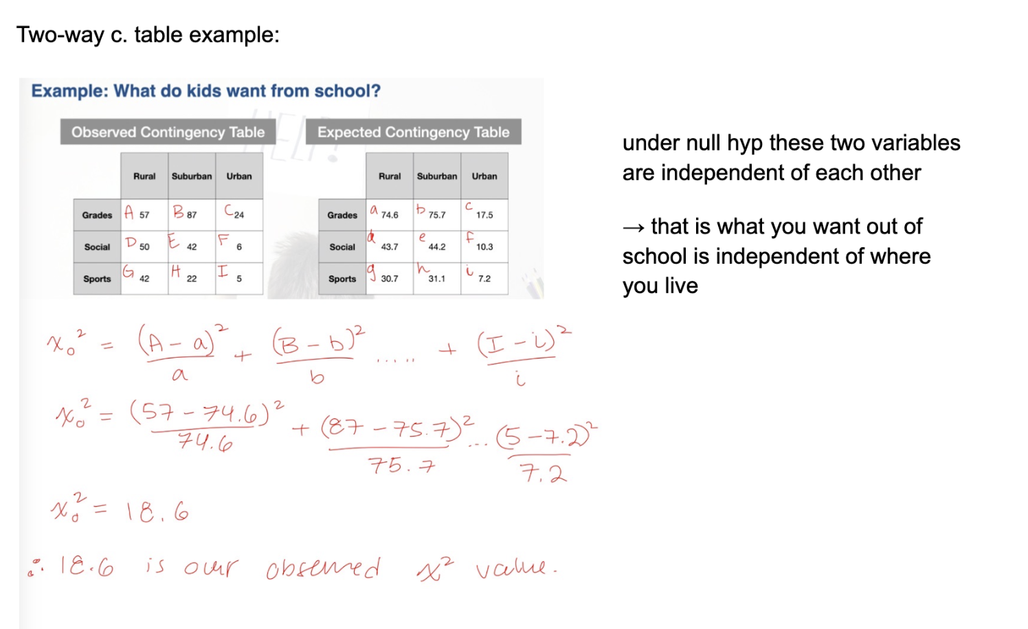
Two-way Contingency Tables:
The research question asks whether the counts are independent between the variables
Example: "Is age independent of year?"
Ho: Worker age and calendar year are independent
HA: Worker age and calendar year are not independent
Expectation: Counts are distributed independently among cells (independently doe NOT mean evenly)
Calculating independence requires first calculating the marginal distribution as proportions
The expected table is the product of the row and column proportions for each cell, multiplied by the table's total
In the context of expected contingency tables, what does an interaction (found between cells) refer to? what information could we gather if the cells were independent?
interaction refers to the cells in the table not having equal relative proportions across the levels of each variable.
if the cells were independent it would mean that the cells in the table have equal relative proportion across levels of each variable.
Chi-squared tests are used to evaluate hypothesis with what type of data?
categorical
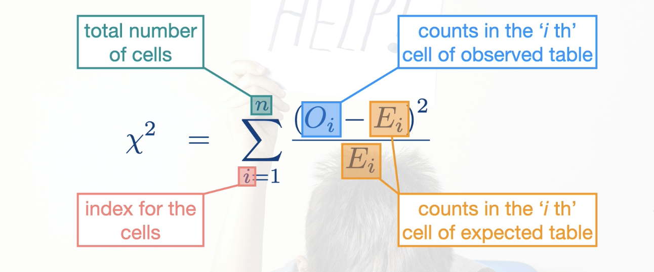
What is the Chi-squared Score?
Chi-squared score: is a measure of the distance between two contingency tables. If the contingency tables are an observed and expected table, then is measures the distance between sample data and the null hypothesis.
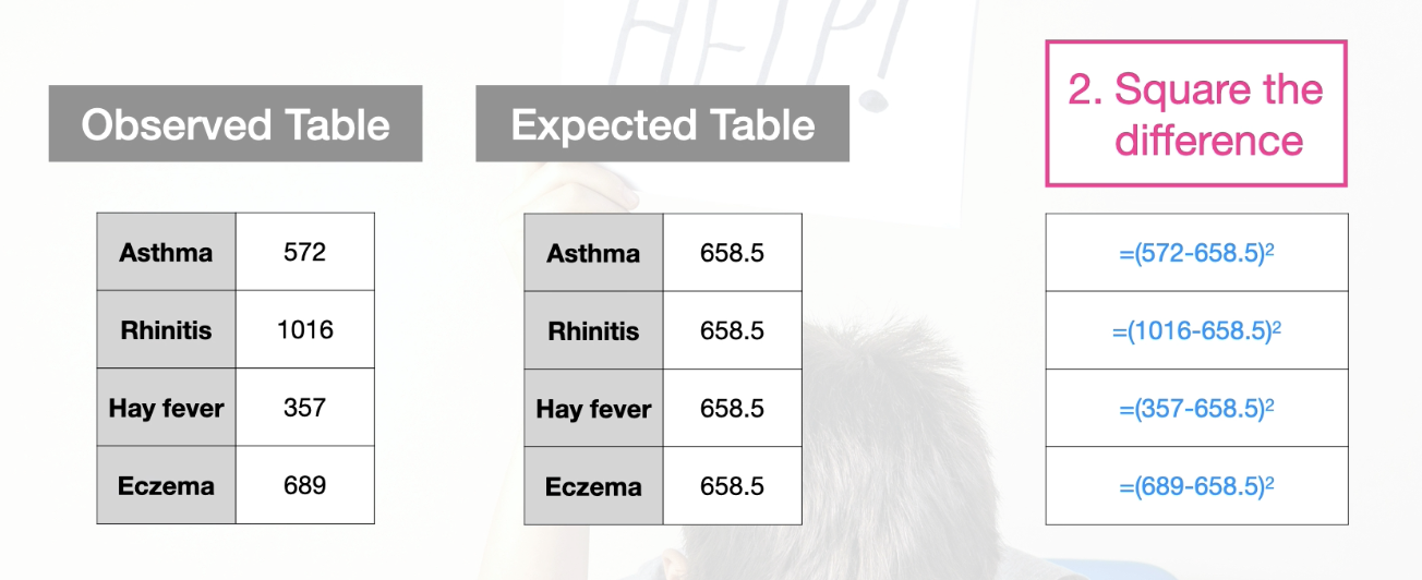
How does the Chi-sqaured score measure distance between observed and expected contingency tables? (4 steps involved)
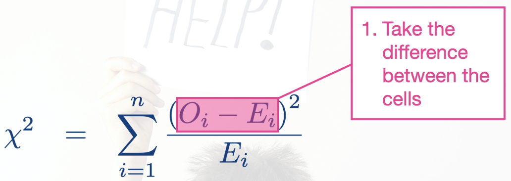
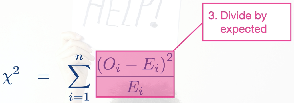
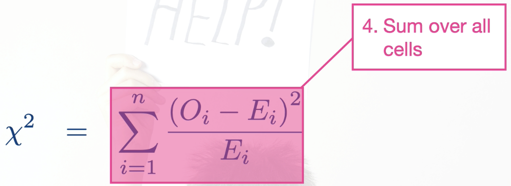
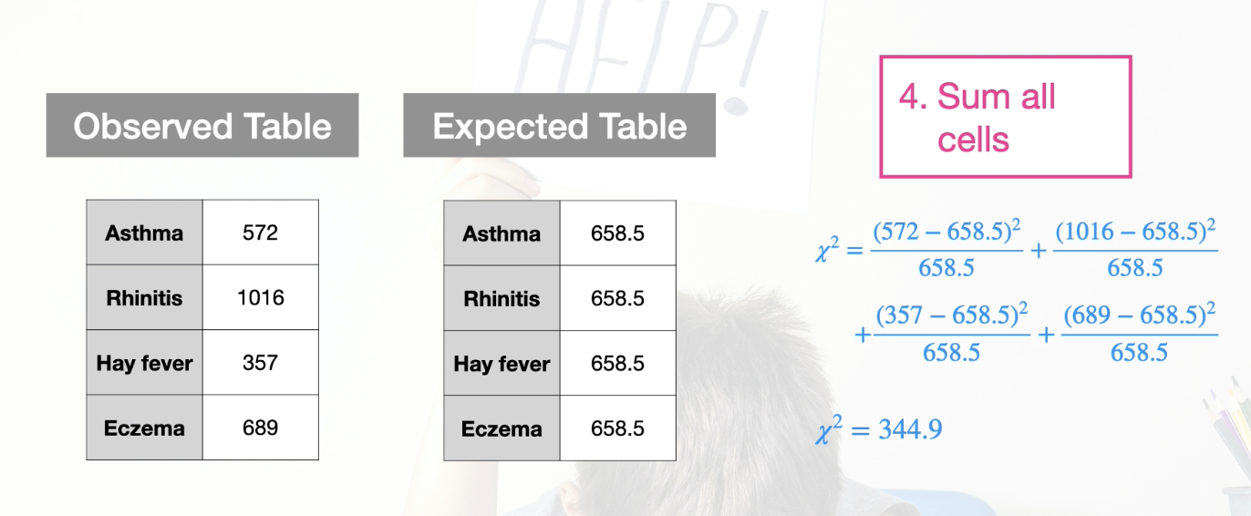
*The four steps are summarized in this mathematical expression:
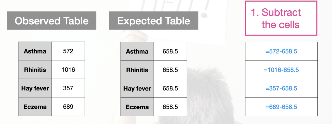
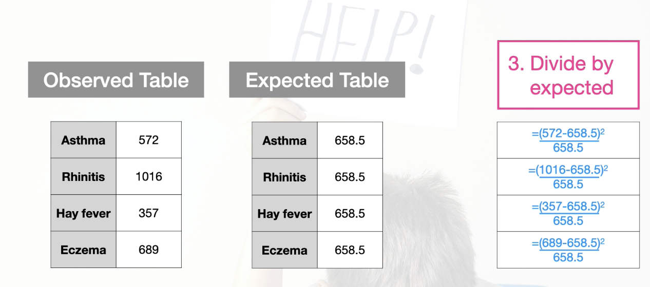
Process: (using 1 way contingency table as example)
Take the difference between each observed and expected cell
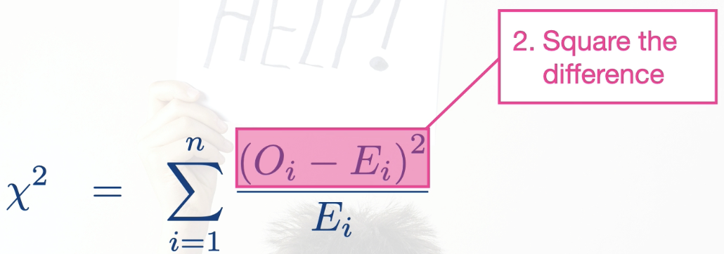
Square the difference
Divide by the expected value
Sum over all cells in the table
Additional example Two Way contingency table process
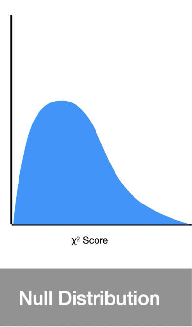
What is a Chi-squared distribution? what does it reperesnt?
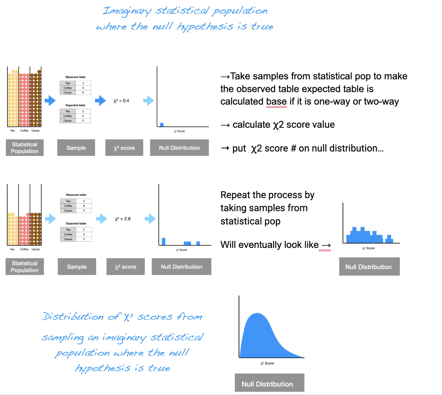
Chi-squared distribution: is the distribution of chi-squared scores expected from repeatedly sampling a statistical population where the null hypothesis was true. It is the null distribution for hypothesis testing with categorical data.
Represents: distribution of chi-squared scores from sampling an imaginary statistical population where the null hypothesis is true.
Chi-squared Hypothesis testing process…
Four Steps:
1)Define the null and alternative hypotheses
Differs between 1-way and 2- way contingency table
1-way: about equality among the cells
2-way: about independence between two categorical variables
2) Establish the null distribution
NOTE: the null hypothesis is embedded in the calculation of the ꭓ2 score
Since null distribution is the chi-squared(ꭓ2) distribution:
The distribution → describes the distribution(or variation in) ꭓ2 scores you would get if you repeatedly sampled a statistical population where the null hypothesis was true.
3) conduct the statistical test
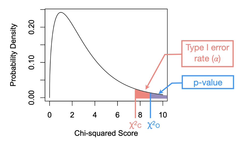
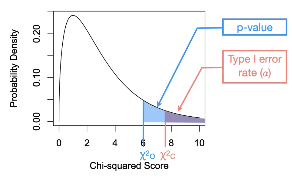
First, we need to locate the Type I error rate(⍺)on the distribution
ꭓ2 c → Chi-squared critical value(*threshold for ⍺)
Threshold is very important! Tells us if we should reject or fail to reject the null hypothesis
ꭓ2O >ꭓ2C
Reject the null hypothesis if the observed score is greater than the critical score.
Or p < ⍺
if the p-value is smaller than the Type I error rate.
ꭓ2O ≤ ꭓ2C
Fail to reject the null hypothesis if the observed score is less than or equal to the critical score.
Or p ≥ ⍺
if the p-value is larger or equal to the Type I error rate.
You must include in the conclusion
Name of the test (ꭓ2)
Degrees of freedom (df)
Total count in the observed table (N=4)
The observed chi-squared value (two decimal places.. In the example below is 3.90)
p-value (three decimal places)
Example: ꭓ2(df=3, N=40)= 3.90; p=0.270
Statement differs for 1-way vs 2-way contingency tables
For 1-way tables, the conclusions are either:
Reject the null hypothesis and conclude that there is evidence to support that the counts are not equal among cells.
Fail to reject the null hypothesis and conclude that there is no evidence to support that the counts are not equal among cells.
For 2-way tables, the conclusions are either:
Reject the null hypothesis and conclude that there is evidence to support that the variables are not independent of each other.
Fail to reject the null hypothesis and conclude that there is no evidence to support that the variables are not independent of each other.
The reporting of a chi-square test should include the following:
Short name of the test (i.e., ꭓ2)
Degrees of freedom
Total count in the observed table
The observed chi-squared value (two decimal places)
p-value (three decimal places)
What makes Correlation tests different from a chi squared test?
(hint type of data)
Chi-squared tests: is a hypothesis test used with categorical data
Correlation tests: are used to evaluate the hypothesis with numerical data
Chi Squared Distribution process…
→Take samples from statistical pop to make the observed table expected table is calculated base if it is one-way or two-way
→ calculate ꭓ2 score value
→ put ꭓ2 score # on null distribution…
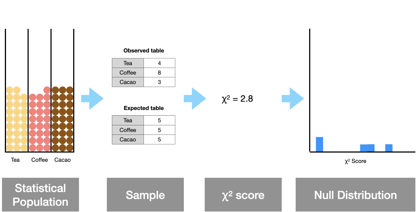
Will eventually be → null distibution
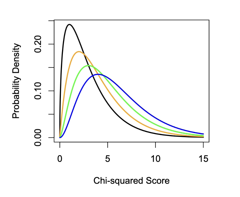
The shape of your size distribution changes slightly with regard to the size of your contingency table(this is due to the degrees of freedom associated with way vs. way contingency tables)
For 1-way tables, the degrees of freedom are df=k-1
When k= # of cells
For 2-way tables, the degrees of freedom are df=(r-1)*(c-1)
When r = # rows, and c = # columns
Here is an example of the Chi-squared distribution for 4 different size contingency tables.
Distitbutions: df=3(black), df=4(orange), df=5(green), df=(blue).
Correlation test defintion
Association defintion
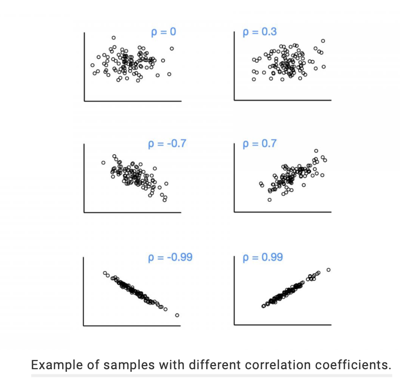
Correlation test: Is the measure of association between two numerical variables. The correlation coefficient can take on values from ⍴=-1, which indicates perfect negative association, to ⍴=0 indicating no association, to ⍴=1 indicating a perfect positive association.
Association: Is a pattern whereby one variable increases (or decreases) with a change in another variable. There is no implied causation between the variables.
Correlation coefficient defintion
Pearson’s correlation coefficient defintion
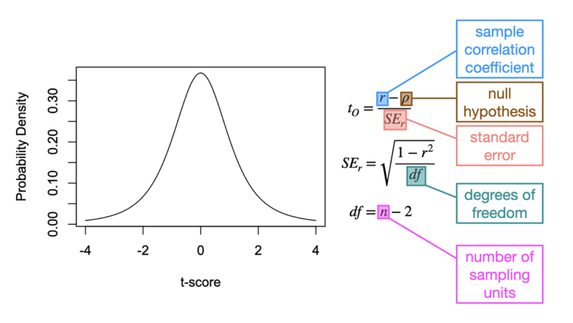
Correlation coefficient: Is the statistical test used to evaluate a sample correlation coefficient against a null hypothesis.
Pearson's correlation coefficient: Is the statistical test used to evaluate a sample correlation coefficient against a null hypothesis.
What are correlation test not used for?
NOT USED FOR PREDICTIONS (linear regressions used for predictions not correlations)
Correlation tests are only used to evaluate the association between variables. They are not used to predict one variable's level based on the other's level.
What range of value could Pearsons correlation coefficent be?
What is r and what is ⍴?
The strength of association is measured using Pearson's correlation coefficient
coefficients can take on values from 1 to -1
r=when correlation is measured from a sample
⍴= when referring to the statical population
Correlations can be thought of as coming from a bivariate normal. concerning correlation strength of association…
What does it mean when ⍴=0 or close to zero?
What does it mean when If ⍴ is negative?
What does it mean when If ⍴ is positive?
What does it mean when ⍴ = ±1
Correlation strength:
If ⍴=0 or close to zero then there is little to no association between variables(x & y-axis)
If ⍴= (-) as you increase one variable the other tends to decrease
If ⍴= (+) as one variable changes the other tends to increase
If ⍴=-1 then it would be a perfect negative association. If ⍴=1 then it would be a perfect positive association.
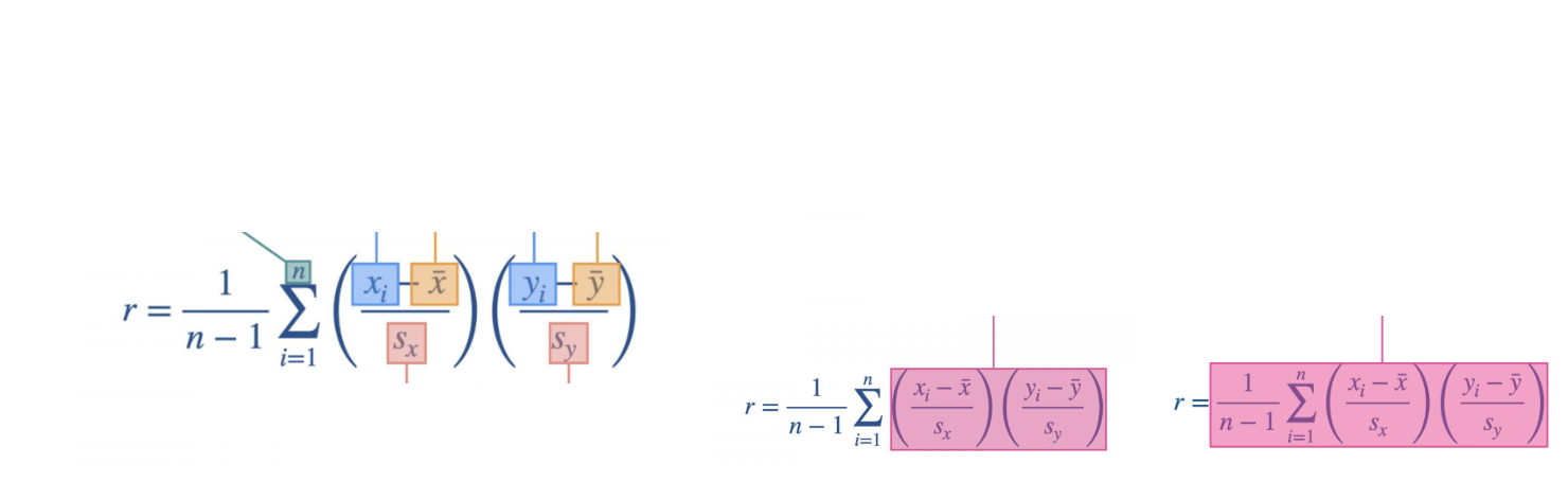
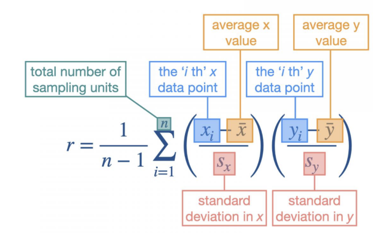
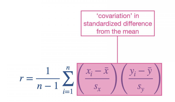
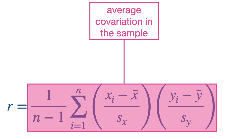
Expression for correlation coefficients:
The xi and the yi have a big influence on the r value. When xi and yi are both positive large numbers(higher than their average mean) the association will be positive. And when one of xi and yi is smaller or negative then you get a negative association value.
Hypothesis Test for correlation…
There is no implied causation between the two variables: looking at the pattern created by variables:
There is no implied causation between the variables. For example, there is a positive association between the arm length and height of people, but one doesn't cause the other.
Both variables are assumed to have variation (but each does not have to be equal amounts of variation)
Both variables are assumed to have variation. We look at this in more detail when learning about linear regression, but correlation tests assume that both variables have comparable amounts of variation among sampling units.
Hypothesis Test:
Define the null and alternative hypotheses
Null and alternative hypothesis (non-directional)
Ho: The correlation coefficient is zero (p=0)
HA: Correlation coefficient, not zero (p≠0)
Null and alternative hypothesis (directional)
Ho: Correlation coefficient is less than or equal to zero (p≤0)
Ho: Correlation coefficient is less than or equal to zero (p≤0)
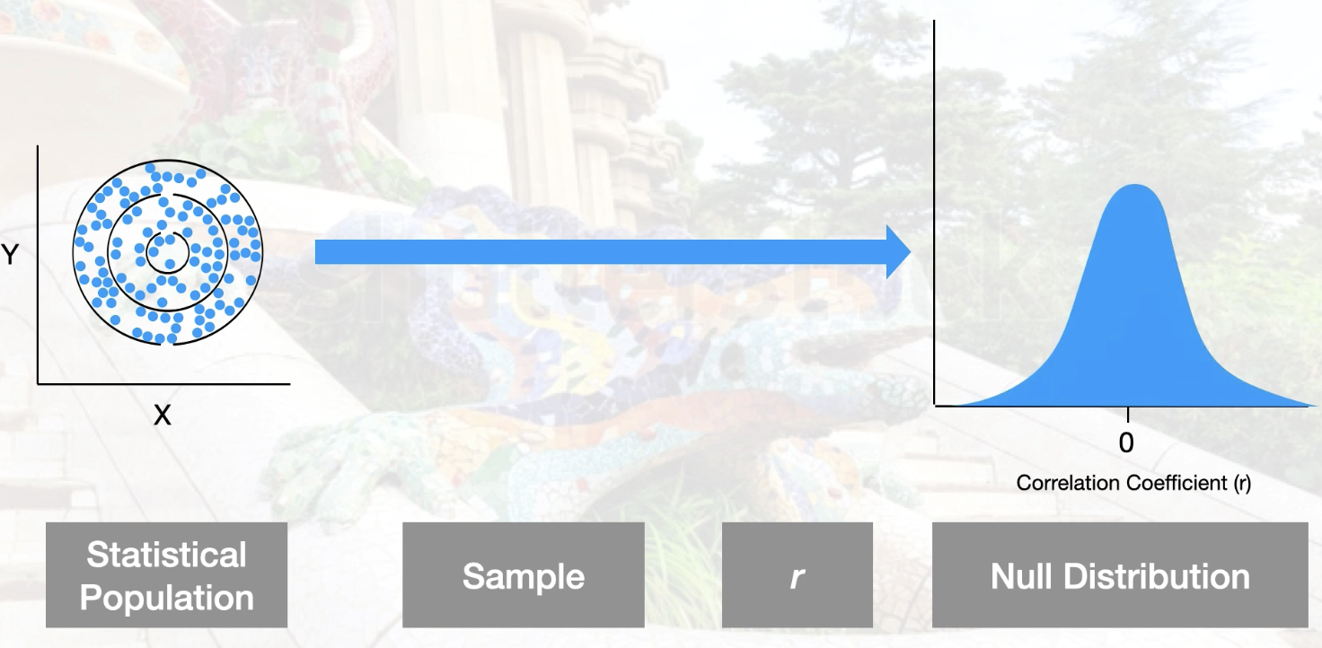
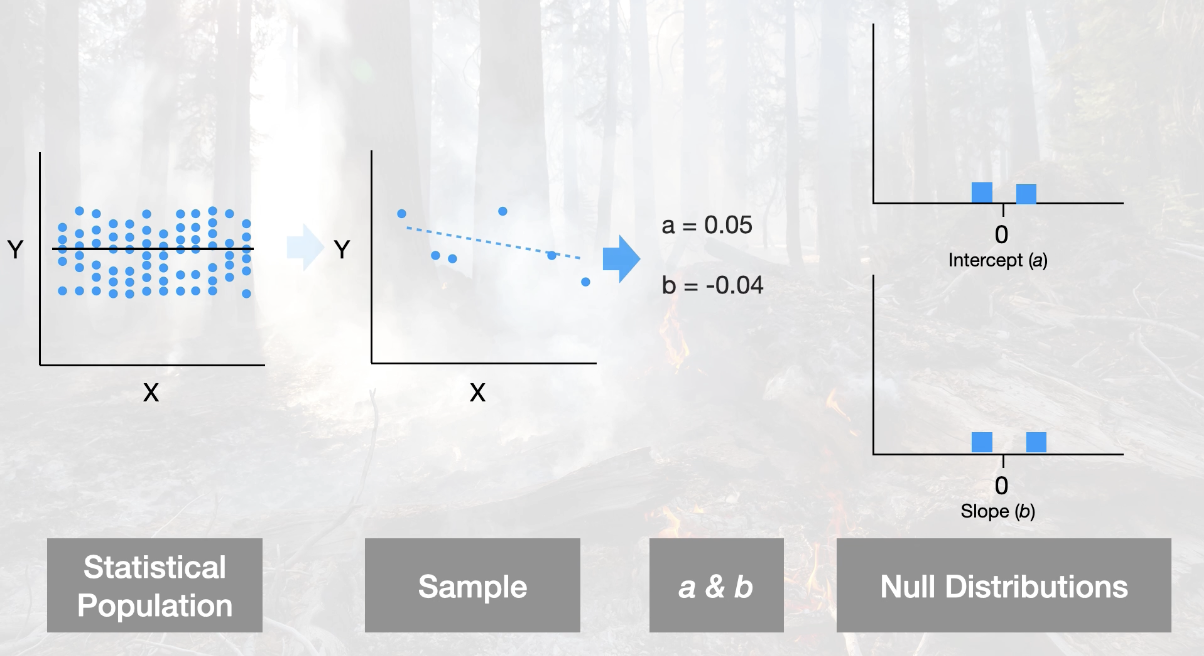
Establish the null distribution
Sampling distribution from repeatedly sampling an imaginary statistical population where the null hypothesis was true
Specifically: sampling distribution of correlation coefficients from a statistical population with no association between variables (i.e., p=0).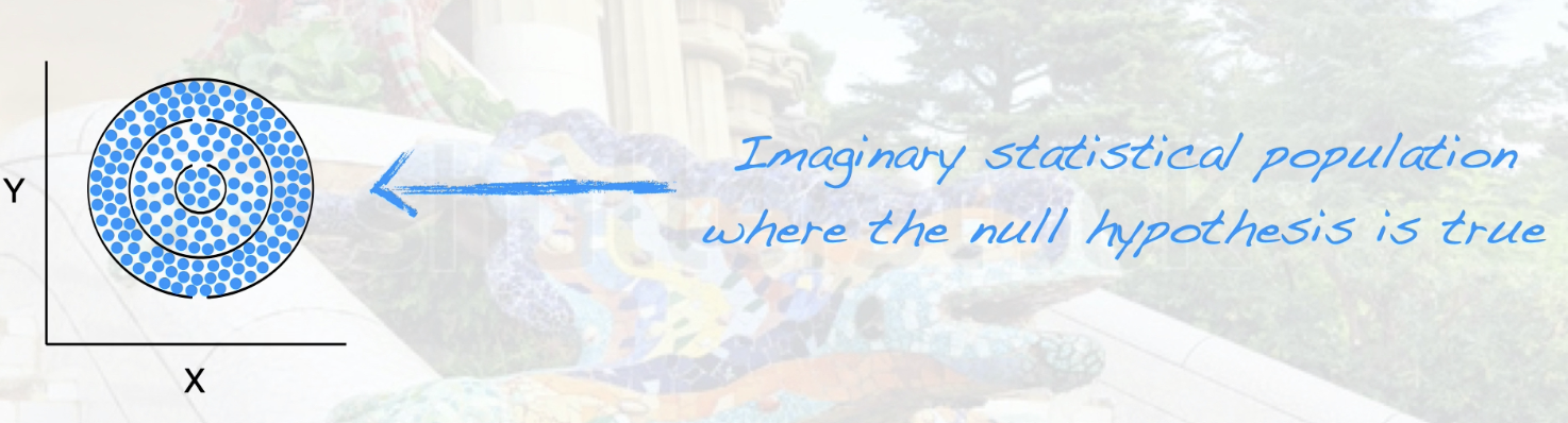
Conduct the statistical test
Locate the observed and critical t-score:
to > tc or p < ⍺
Reject the null hypothesis → if the observed score is greater than the critical score (i.e., to>tc) or if the p-value is smaller than the Type I error rate (i.e.,
p<a).
to ≤ tc or p ≥ ⍺
Fail to reject the null hypothesis → if the observed score is less than or equal to the critical score (i.e., to ≤ tc) or if the p-value is larger or equal to the Type I error rate (i.e., p≥⍺)
Draw scientific conclusions
For non-directional hypotheses, the conclusion is either:
Reject the null hypothesis and conclude there is evidence of an association.
Fail to reject the null hypothesis and conclude there is no evidence of an association.
For directional hypotheses, the conclusion is either:
Reject the null hypothesis and conclude there is evidence of a positive (or negative) association.
Fail to reject the null hypothesis and conclude there is no evidence of a positive (or negative)
Reporting of correlation test should include the following:
Symbol for the test (i.e., r)
Degrees of freedom
Observed correlation value (two decimal places)
p-value (three decimal places)
Example: Pearson correlation, (96)=-0.656,
What is linear regression?
Linear regression: Is the statistical test used to evaluate whether changes in one numerical variable can predict changes in a second numerical variable
Structure of linear regression…
how does this differ for experiment studies vs observational studies.
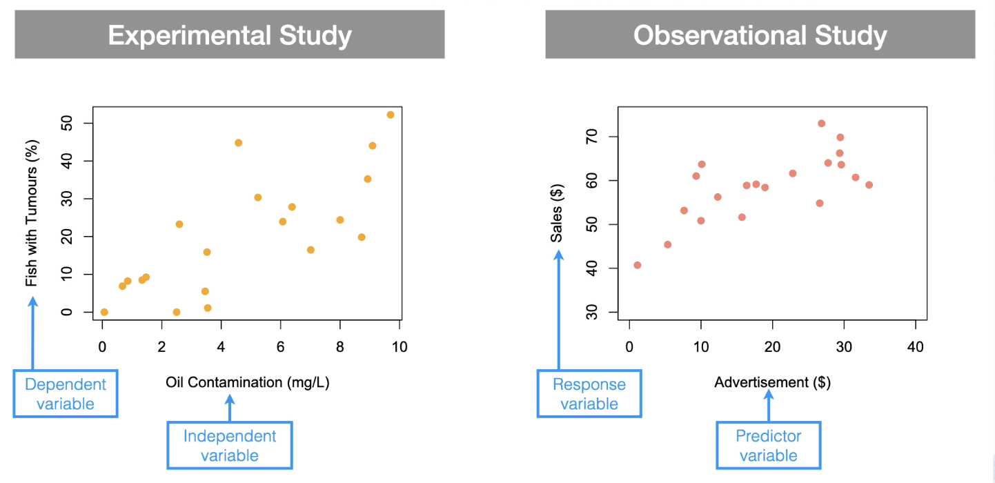
Structure of Linear Regression:
The focus of linear regression is prediction
One variable is the predictor variable and the other is the response
variable
For experimental studies, the predictor variable is what was manipulated, and is called the independent variable. The response variable called the dependent variable.
For observational studies, the choice of predictor versus response variable depends on the research
What does each of the variables represent?
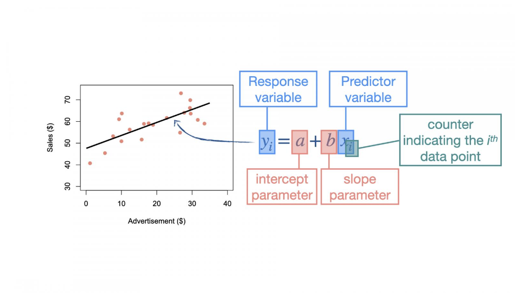
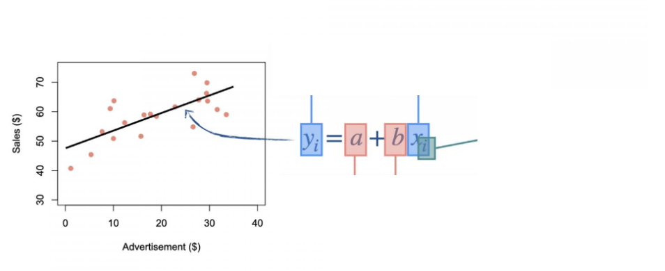
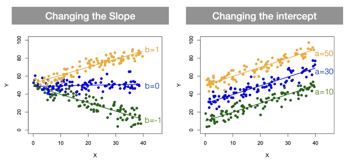
Slope (b) is the amount that the response variable (y) increases (or decreases) for every unit change in the predictor variable (x).
Intercept (a) is the value of the response variable (y) when the predictor variable (x) is at zero (i.e., x=0).
How would changing the slope effect the graph?
How would changing the intercept effect the intercept?
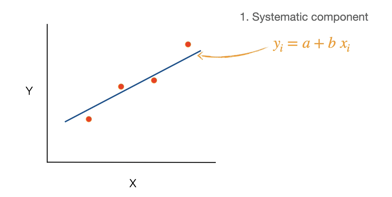
What is the systemic component?
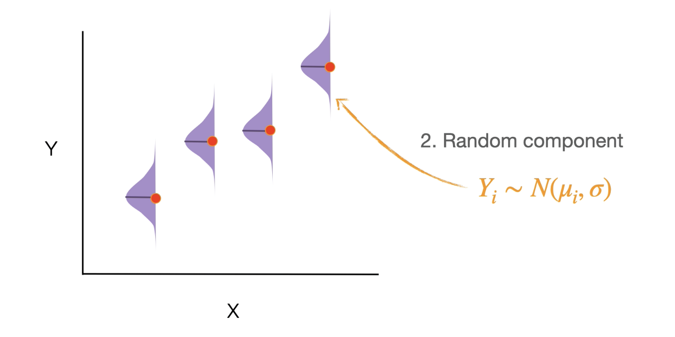
What is the random component?
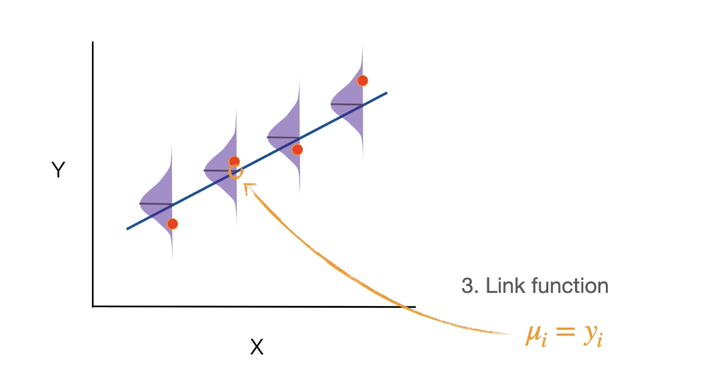
What function connects these two components?
The systematic component describes the mathematical function used for predictions.
Systematic component is the linear equation used to make a prediction
Random component describes the probability distribution for sampling error. For linear regression, this is a Normal distribution.
Random component refers to the eros distribution that decides the sampling error - for linear regression the assumptions are: our sampling error only occurs int he y variable(the response variable) NEVER occurs in predictor variables. Also assumed our data Yi is are distributed b a normal distribution with a mean(mu,i) and a standard deviation(sigma) mu has a ‘i’ because mean can vary but sigma has no i so that means we assume equal variance no matter where you are on the x axis. Standard deviation doesn’t change only mean.
*The link function connects the systematic component to the random component.
Binds systematic component with random component by saying that the mean of the systematic component and the mean of the random component are the same.
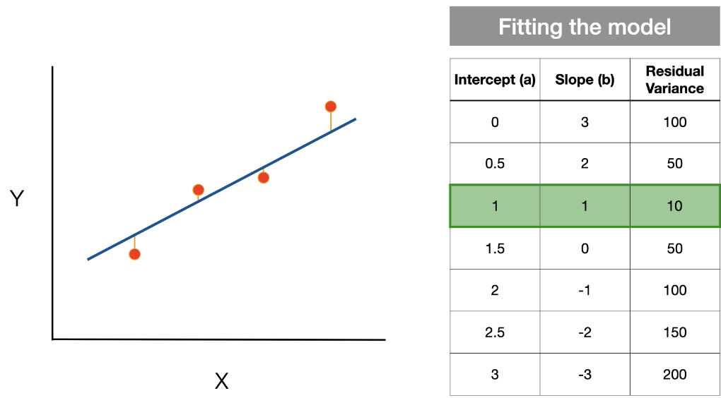
Fitting the statistical model to data
Fitting the model means estimating the intercept and slope that best
explain the data.
Minimizing the residual variance or 'sums of squares’
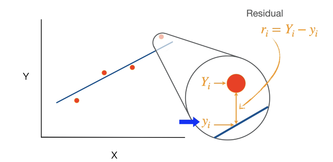
What does each vaule in the equation represent?
Residual is the difference between an observed data point(Yi) and the predicted value at the x location(yi). Little ri rerepsents the residual… this is ddiferne than other little r.
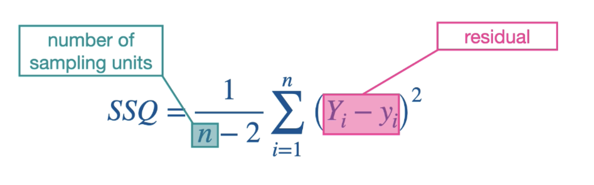
Calculate the residual for each data point
Take the square of each residual
Sum the squared residuals across all data points
Divide by the degrees of
***little orange lines represent the residuals(ri)**
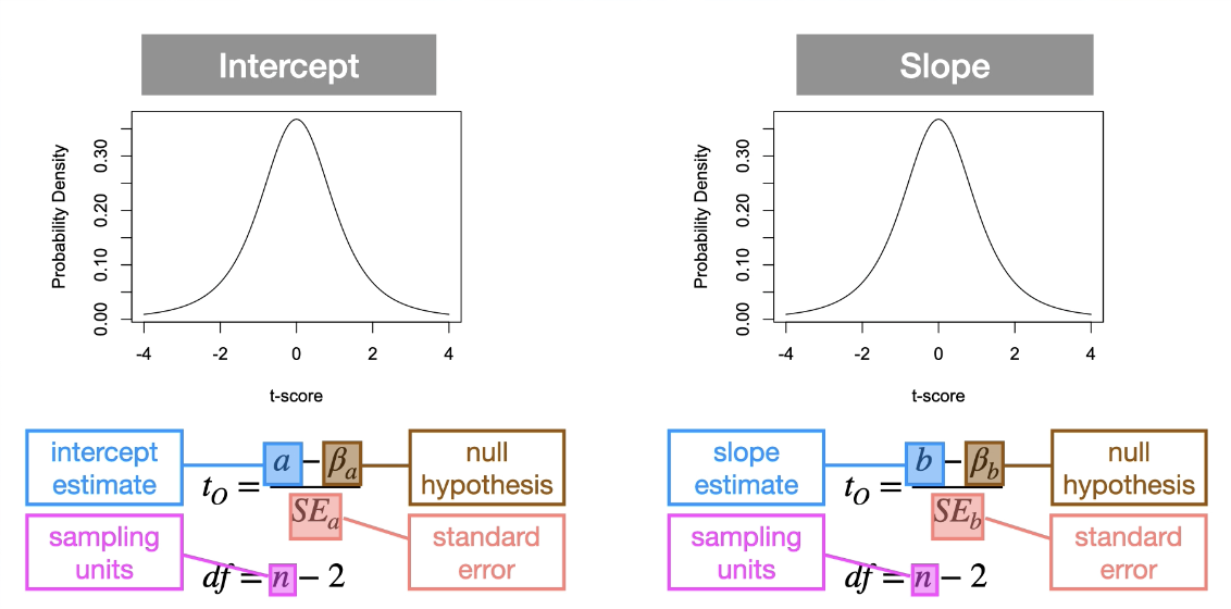
Linear regression Hypothesis test….
Hypothesis Testing on Slope and Intercept:
*two hypothesis tests for each intercept and slope:
1. Define the Null and Alternative Hypothesis:
INTERCEPT (a)
Used to answer questions at the specific point of x=0.
Ie "What do my instruments detect when there is no contaminant present in the water"
How does the intercept (a) relate to a reference value
Using a to represent the estimated intercept, and βa to represent a reference value of interest, the non-directional null and alternative hypothesis is
HO: Intercept
(is not different from a reference value, or a=βa in symbols)
HA: Intercept
(is different from a reference value, or a≠βa in symbols)
An example of a directional null and alternative hypothesis is
HO: a≤βa
HA: a>βa
SLOPE (b)
More common
Used to answer questions about how much y changes with one unit change
in X.
Ie "How much does the level of iron in the blood change with each unit change in iron
Using b to represent the estimated slope, and βb to represent a reference value of interest, the non-directional null and alternative hypothesis is
HO: Slope
(is not different from a reference value, or b=βb in symbols)
HA: Slope
(is different from a reference value, or b≠βb in symbols)
An example of a directional null and alternative hypothesis is
HO: b≤βb
HA: b>βb
2. Establish the Null distribution:
Repeat sampling until null is established
Since our two null distributions are t-distributions we will be able to do a two-sample t-test!!
Null distribution is a sampling from a statistical population where the null is true.
Since estimating the standard deviation from a sample, null
distribution is a t-distribution
3.Conduct statistical test:
Compare the Type I error rate (a) against the p-value (p).
Type I error rate is the probability of rejecting the null hypothesis when it is true.
The p-value is the probability of observing your data, or something more extreme, under the null hypothesis
Obtaining p-vaule using computer software.
Calculate t-observed for each intercept and slope (WE CANNOT CALCULATE STANDARD ERROR BY HAND)
Conduct the statistical test:
Locate the observed and critical t-score:
to > tc or p < ⍺
Reject the null hypothesis → if the observed score is greater than the critical score (i.e., to>tc) or if the p-value is smaller than the Type I error rate (i.e.,
p<a).
to ≤ tc or p ≥ ⍺
Fail to reject the null hypothesis → if the observed score is less than or equal to the critical score (i.e., to ≤ tc) or if the p-value is larger or equal to the Type I error rate (i.e., p≥⍺)
4. Draw scientific conclusions: difference for slope and intercept
Intercept:
If we reject the null hypothesis, we could write: "Reject the null hypothesis and conclude there is evidence that the predicted response variable is different from the reference (Ba) at x=0."
If we fail to reject the null hypothesis, we could write: "Fail to reject and conclude there is no evidence that the predicted response variable is different from the reference (Ba) at x=0”
Slope:
If we reject the null hypothesis, we could write: "Reject the null hypothesis and conclude there is evidence that changes in the predictor variable predict changes in the response variable that are different than the reference value (Bb)."
If we fail to reject the null hypothesis, we could write: "Fail to reject the null hypothesis and conclude there is no evidence that changes in the predictor variable predict changes in the response variable that are different than the reference value (Bb).”
The reporting of a linear regression should include:
Symbol for the parameter being tested (i.e., a or b)
Observed parameter value (two decimal places)
Observed t-score
Degrees of freedom
p-value (three decimal places)
Linear regression assumptions…. what are these assumptions? and what are their definitions? (4)
There are four main assumptions for a linear regression:
Linearity: The response variable(y variable) should well described by a linear combination of the predictor variable(x variable).
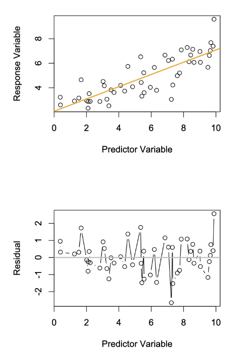
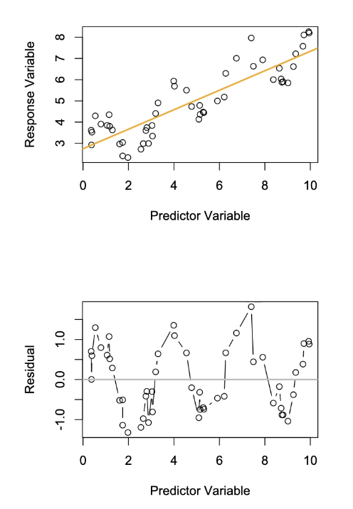
Independence: The residuals along the predictor variable should be independent of each other.
Normality: The residual variation should be Normally distributed. DATA does NOT have to be normally distributed just the Residuals
Homoscedasticity: The residual variation should be similar(about the same) across the range of the predictor variable(x variable).
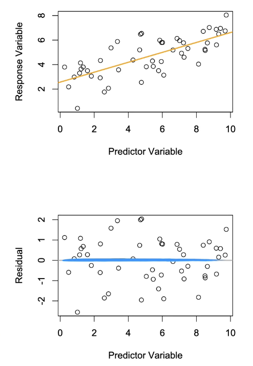
In the graphs below when is the assumption of linearity met and when is it not?
Linearity:
response variable is a linear combination of the predictor variable
For simple linear regression (y=a+bx), it is a straight line
Evaluated good relationship between preditocr and reposense:
we evaluate qualitatively by graph of residuals against the predictor variable
Assumption of Linearity is Met:
This figure shows data from the predictor variable and response variable:
Orange: Fit line is shown in orange → You can see for higher levels of predictor variable that your response variable increases as well.
Blue: This residual graph represents the distance from the data points to your predicted line. This plot is the residuals against the predicted value. Looking for the obvious trend in predictor value or an average of x. Represented by blue line
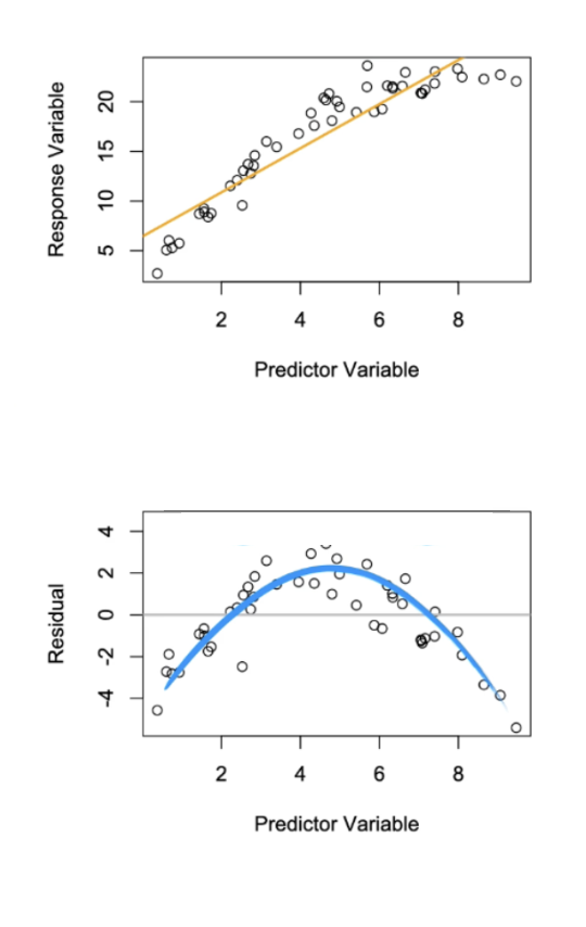
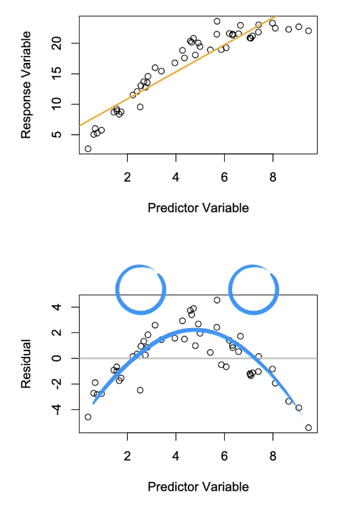
When Assumption of Linearity is Violated:
Orange: Data points do not follow a trend. So when we put in fit line shown in orange there is places where the values are less than the line at the beginning and then above and then below again. That is the pattern the residuals are looking at detecting….
Blue: So when we plot residuals against predictors we see a clear pattern. This will either be a frowning curve or a happy curve depending on the change in values on the original graph either one we don’t want.
In the graphs below when is assumption of independence met and when is it not?
Independence:
Residuals are independent from each other
Can be violated if there is some unknown spatial or temporal relationship
among the sampling units.
Prevent by ensuring that sampling units are selected at random and independently of each
Evaluated qualitatively using a plot of residuals against the predictor variable.
Assumption of Independence is Met:
Orange: The same data used as previous
Grey: Can see that the residuals are independent of each other because there is no pattern and they just flip sign with one another
When Assumption of Independence is Violated:
Orange: Patterning in the first graph is inductor but can only be fully seen in residuals
Grey: In residuals, it can be seen there is a pattern of samples and they were not selected independently of each other.
In the graphs below when is assumption of Normality met and when is it not?
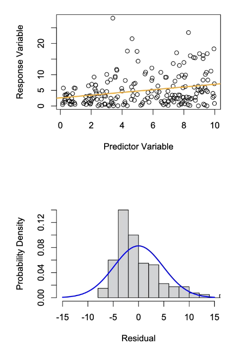
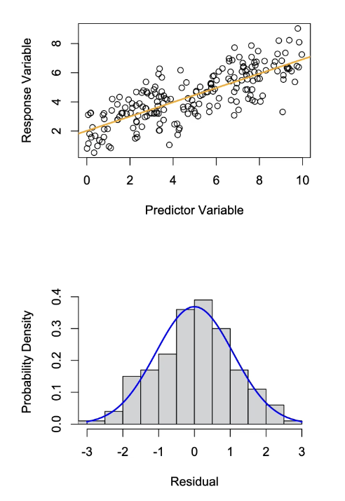
Normality:
Residuals are normally distributed (the data is typically never normally distributed)
Violations can be caused by an unusual statistical population or a consequence of violations of linearity.
Evaluated qualitatively using a histogram of residuals and a reference
normal distribution.
Evaluated quantitatively using the Shapiro-Wilks
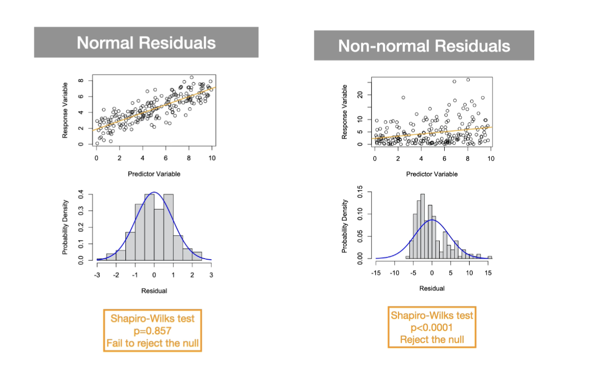
Assumption of Normality is Met:
Orange: The fit regression line is shown in orange and in this data set the assumption of normality is met.
Blue: Histogram of residual values. Relatively symmetrical and roughly has a bell shape. Then we compare to normal distribution
When Assumption of Normality is Violated:
Orange: The fit line is shown in orange
Blue: Long tail on one side and not the other
Superimpose null distribution - we can see that the residuals are not normally distributed.
What is the Shapiro-Wilks assumption test of normality?
When do we fail to reject?
When do we reject?
Shapiro-Wilks Test: Statistical test used to quantitatively evaluate the assumption that the residuals are normally distributed.
Normality Shapiro-Wilks test:
The null and alternative hypotheses are:
Ho: The residuals are normally distributed
HA: The residuals are not normally distributed
If p ≥ ⍺ then we fail to reject the null hypothesis and conclude that there is no evidence to say that the residuals are not normally distributed.
If p < ⍺ then we reject the null hypothesis and conclude that there is evidence to say that the residuals are not normally distributed.
p is greater than or equal to ⍺= 0.05 p is less than or equal to ⍺= 0.05