Chapter 7: The Central Limit Theorem
Introductory
Central limit theorem: If the sample size is large enough then we can assume it has an approximately normal distribution.
The sample size has to be greater than 30 to assume an approximately normal distribution
Exponential Distribution: a continuous random variable (RV) that appears when we are interested in the intervals of time between some random events
7.1 The Central Limit Theorem for Sample Means (Averages)
μX = the mean of X
σX = the standard deviation of X
𝑥¯ ~ N**(𝜇𝑥, 𝜎𝑋 / 𝑛√)** = If you draw random samples of size n, then as n increases, the random variable 𝑥 which consists of sample means, tends to be normally distributed
sampling distribution of the mean: approaches a normal distribution as n, the sample size, increases.
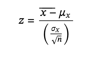
The random variable 𝑥¯ has a different z-score associated with it from that of the random variable X. The mean 𝑥¯ is the value of 𝑥¯ in one sample.
μX = the average of both X and x¯
Standard error of the mean: 𝜎𝑥 = 𝜎𝑋 / √𝑛 =standard deviation of x¯
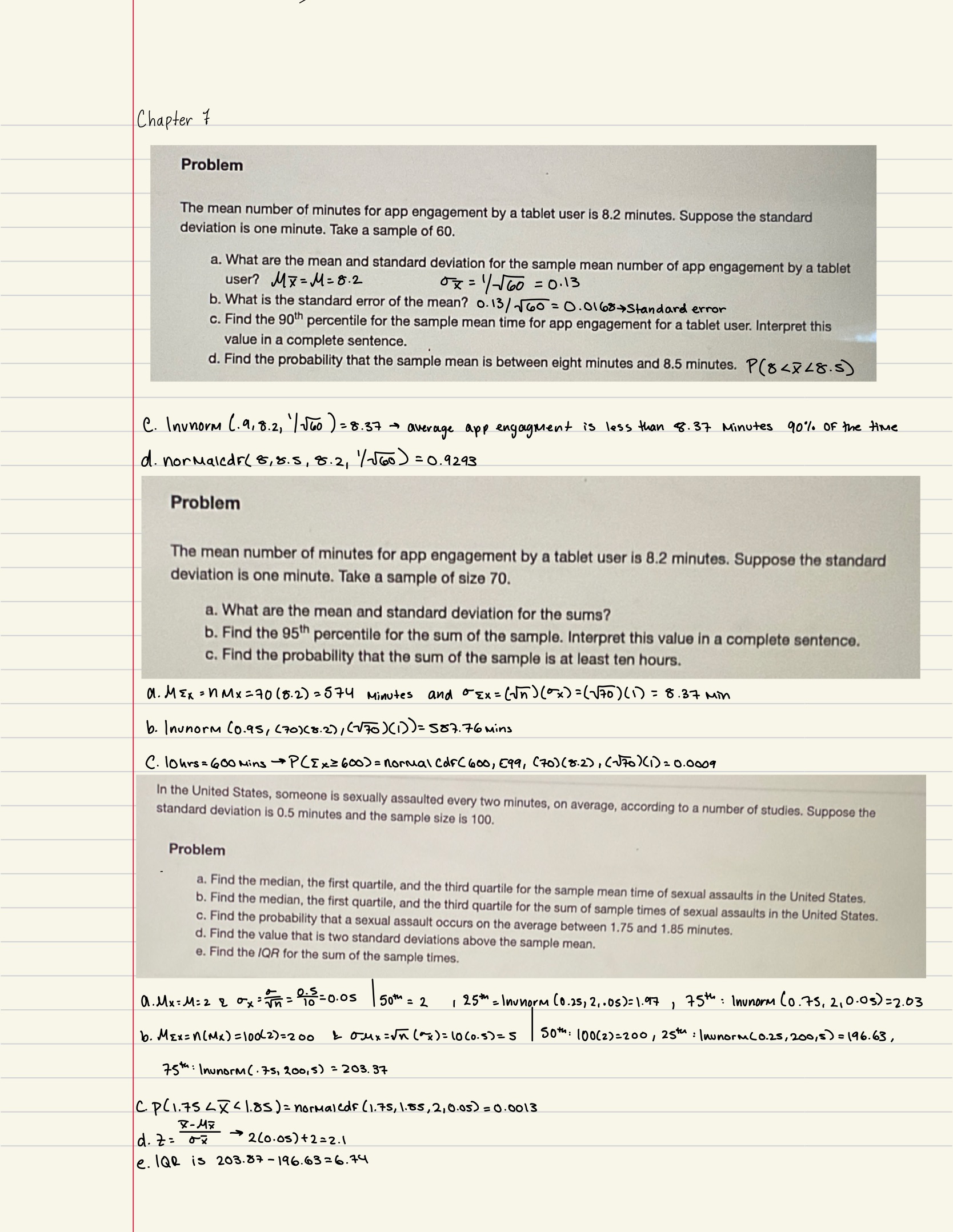
Probabilities for means on the calculator
2nd DISTR
2:normalcdf
normalcdf (lower value of the area, upper value of the area, mean, standard deviation / √sample size)
where
mean is the mean of the original distribution
standard deviation is the standard deviation of the original distribution
sample size = n
Percentiles for means on the calculator
2nd DISTR
3:InvNorm
k = invNorm (area to the left of 𝑘, mean, standard deviation / √sample size)
Where→
k = the kth percentile
mean is the mean of the original distribution
standard deviation is the standard deviation of the original distribution
sample size = n
7.2 The Central Limit Theorem for Sums
The central limit theorem for sums: As sample sizes increase, the distribution of means more closely follows the normal distribution.
∑X ~ N[(n)(μx),(𝑛√n)(σx)]
The normal distribution: has a mean equal to the original mean multiplied by the sample size and a standard deviation equal to the original standard deviation multiplied by the square root of the sample size**.**
The random variable ΣX has the following z-score associated with it:
Σx is one sum.
𝑧 = 𝛴𝑥–(𝑛)(𝜇𝑋) / (√𝑛)(𝜎𝑋)
(n)(μX) = the mean of ΣX
(√n)(𝜎X) = standard deviation of ΣX
Probabilities for sums on the calculator
2nd DISTR
2: normalcdf (lower value of the area, upper value of the area, (n)(mean), (√n)(standard deviation))
where:
mean is the mean of the original distribution
standard deviation is the standard deviation of the original distribution
sample size = n
Percentiles for sums on the calculator
2nd DIStR
3:invNorm
k = invNorm (area to the left of k, (n)(mean), (√n)(standard deviation)
where:
k is the kth percentile
mean is the mean of the original distribution
standard deviation is the standard deviation of the original distribution
sample size = n
7.3 Using the Central Limit Theorem
Law of large numbers: if you take samples of larger and larger size from any population, then the mean x¯ of the sample tends to get closer and closer to μ.
Binomial distribution:
there are a certain number n of independent trials
the outcomes of any trial are success or failure
each trial has the same probability of a successful p
Examples